NOBODY has time for 243 experiments: Try CCD

Dec 21

Why two-level designs aren’t enough

So far, we’ve gone over the basics of two-level full factorial and fractional factorial designs. They’re great, but they hit a wall when we’re dealing with non-linear relationships, trying to find the maximum or minimum of a system, or looking for that perfect “sweet spot.” Sure, we could use full factorial designs with three or more levels, but the number of experiments would get out of hand really quickly.

    
            Number of Factors
            3-Level Full Factorial Runs
            Central Composite Design (CCD) Runs
        
            2
            9
            16
        
            3
            27
            22
        
            4
            81
            32
        
            5
            243
            50

What Central Composite Design (CCD) is

A Central Composite Design (CCD) is much better suited for this. It’s part of response surface methodology and works by adding a few extra design points—center points in the middle of the design and star-like axial points around it. This lets us capture quadratic effects without running as many experiments as a three-level full factorial design would need.

An optimization example

Let’s look at an example where we’re trying to optimize the yield of a chemical reaction. Using Central Composite Design (CCD), we’ll figure out the best combination of two factors—time and temperature—to hit that sweet spot where the yield is at its maximum.

The table below shows the design plan. To keep things simple, we’ve encoded the variables. The orange rows show the basic 2x2 factorial design that forms the foundation. On top of that, we’ve added center points (marked in purple) and star points (in dark blue). The star points are positioned at a distance of ±α from the center, where α represents the square root of the number of factors. The experiments have already been run, and we’ve recorded the yield for each setup. Let’s see what we’ve got!

Visualize the data

The scatterplot below provides an overview of the results. On the left, we see how time affects the average yield, with the center point showing a peak in the curve. On the right, we have temperature, which shows a similar pattern. Both plots show a clear curvature, something a simple 2x2 factorial or fractional design wouldn’t have captured.

Model building and refinement

The scatterplots above provided a clear indication of the key model parameters, particularly emphasizing the importance of the quadratic terms. The ANOVA table below confirms that. The quadratic terms are highly significant and the only insignificant parameter is the time:temperature interaction that we exclude from the model.

Below we see the model together with the measured data. The predictions seem to align reasonably well with the observed data and we can use that fit to determine the maximum yield.

Finding the optimum region with a contour plot

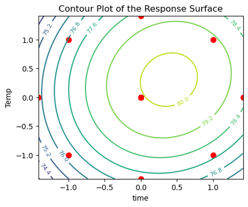
A contour plot helps us to visually pinpoint the best settings for temperature and time. In this case, the plot shows that the maximum yield—around 80—occurs when both factors are close to 0.5.

While we wouldn’t have been able to capture this with just a two-level full factorial or fractional design, those designs are still crucial for narrowing down the number of factors to a manageable level.

Give it a try yourself! In the next blog post, I’ll show you how to create a central composite design in Python.

Marcel Butschle