
Testing Bayesian Optimization for Lab Experiments
Bayesian Optimization promises to make experimental design smarter and more efficient by iteratively selecting the most promising experiments based on previous results. But how do we know if it’s actually better than simpler approaches?
In this post, I put it to the test using real lab data. We’ll see how it compares against random sampling and fractional factorial design.
1. The Experiment: Optimizing Material Properties
The test case involves optimizing the hardness of a coating. The data comes from a student project where they performed a 2-level full factorial design with six factors (total of 64 runs):
- Curing Temperature
- Pigment Volume Concentration
- Catalyst Concentration
- Cross-linking Density
- Catalyst-Type
- Hardener
I used coded values (-1 and +1) for simplicity. Here’s a look at the first few runs:
| Run Order | Temp (coded) | PVC (coded) | Catalyst Conc (coded) | Crosslinking (coded) | Catalyst Type (coded) | Hardener Type (coded) | Pendulum Hardness |
|---|---|---|---|---|---|---|---|
| 1 | -1 | 1 | -1 | -1 | -1 | 1 | 71 |
| 2 | 1 | 1 | -1 | -1 | -1 | 1 | 98 |
| 3 | -1 | 1 | -1 | 1 | -1 | 1 | 78 |
| 4 | 1 | 1 | -1 | 1 | -1 | 1 | 99 |
| 5 | -1 | 1 | -1 | -1 | -1 | -1 | 69 |
| 6 | 1 | 1 | -1 | -1 | -1 | -1 |
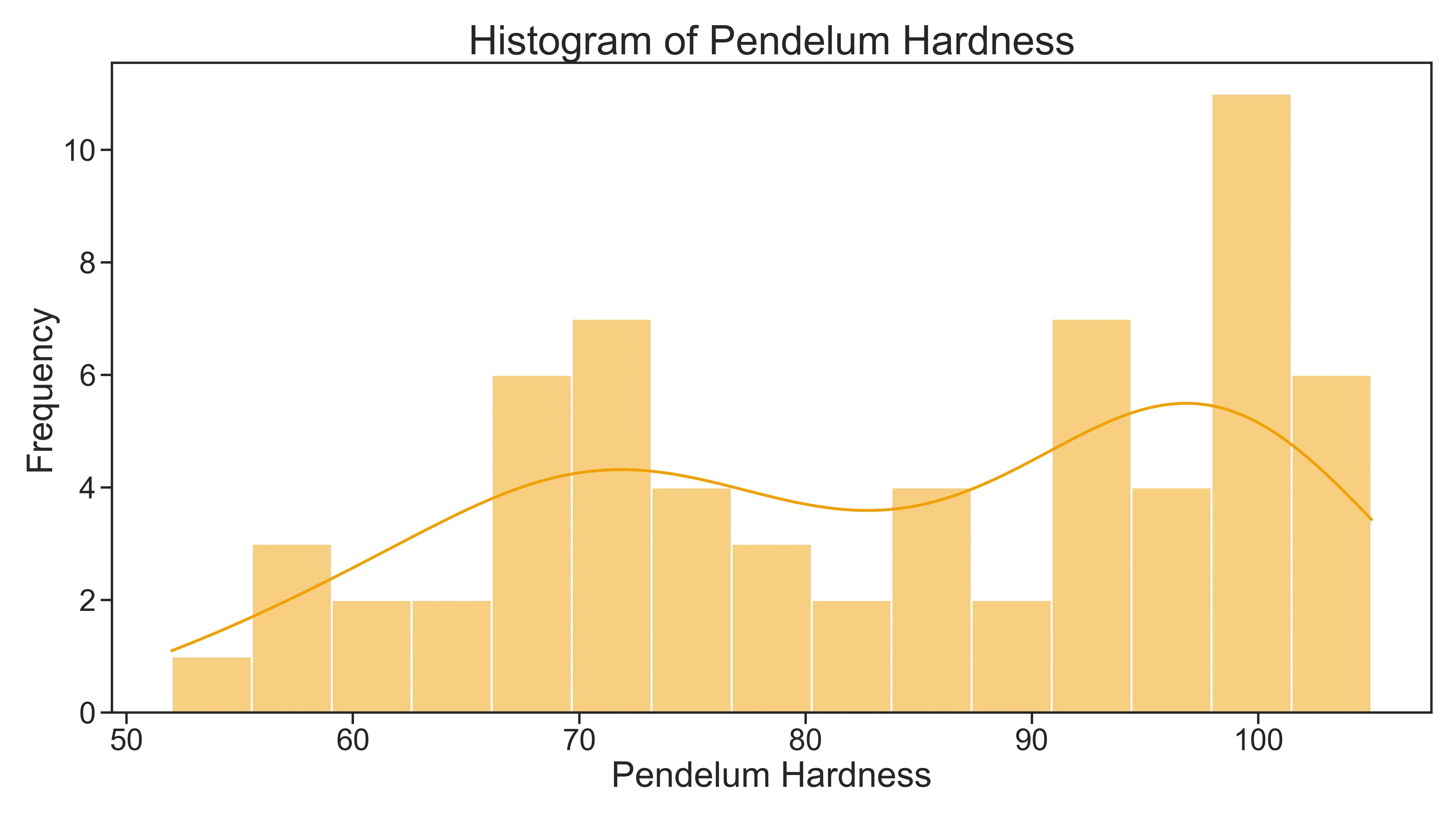
As I said, the goal was to optimize pendulum hardness. Let’s take a quick look at the distribution. You’ll notice a kind of bimodal pattern, with many values clustering around 70 and another peak around 100:
2. Defining the Baseline: Random Sampling
Before jumping into Bayesian Optimization we need to establish a baseline: how well could we do by simply picking experiments at random? This helps us evaluate the performance of the algorithm later.
To quantify this, I performed a simple simulation:
- In each iteration, 10 samples were drawn randomly (without replacement) from the dataset.
- For each set, I recorded the maximum observed pendulum hardness.
- This process was repeated 100,000 times to estimate the probability of exceeding various performance thresholds by chance.
Here are the results:
| Threshold | Probability max(sample) > threshold | N datapoints above threshold |
|---|---|---|
| 90 | 99.82% | 28 |
| 100 | 71.73% | 7 |
| 101 | 65.72% | 6 |
| 102 | 50.38% | 4 |
| 103 | 15.73% | 1 |
This tells us that it is pretty easy to get above 90. If we just perform 10 random experiments from the full factorial design, basically always we would observe hardness values above 90. For higher thresholds (above 100), the probability drops: only about half the random samples reach above 102, and just 16% exceed 103. This baseline shows that while it’s easy to find “good” results by chance, finding the very best results is much less likely without guidance.
4. Setting the Bar: What Counts as “Success”?
To meaningfully evaluate optimization performance, we need to focus on outcomes that are truly difficult to achieve by chance. As shown in the random sampling baseline, values above 102 are rarely reached through random selection—only about 50% of random campaigns exceed this threshold, and even fewer surpass higher values. By setting the threshold above 102, we ensure that “success” reflects genuine optimization skill rather than luck, making it a much more stringent and informative benchmark for comparing algorithms.
5. Bayesian Optimization in Practice: The BayBE Algorithm
To put Bayesian Optimization to the test, I used the BayBE package. I am not going into details here. You can find the documentation here and I also provide the complete code and data on my GitHub.
You only need to know that each optimization campaign consists of several rounds (cycles), where in each round a batch of new experiments is recommended and evaluated. The two main parameters controlling the campaign are:
- BATCH_SIZE: The number of new experiments (suggestions) proposed in each round.
- N_CYCLES: The total number of rounds (iterations) in a campaign.
For example, with BATCH_SIZE = 2 and N_CYCLES = 5, each campaign evaluates 10 experiments in total (same as in our simulation).
6. Comparing Results: BayBE vs. Random Sampling
To assess the practical benefit of Bayesian Optimization, I ran 100 independent optimization campaigns using (1) a random recommender and (2) the BayBE recommender (with a Random Forest surrogate model). For the random recommender we expect that only in 50 out of the 100 campaigns we measure a pendulum hardness above 102. With the BayBE recommender we need to be much better than that to call it a success.
Here are the results:
- Random recommender: Exceeded the threshold in 47 out of 100 campaigns (similar as what we expected from our simulation).
- Bayesian recommender (BayBE): Exceeded the threshold in 98 out of 100 campaigns.
Wow! With just 10 out of 64 total experiments, it almost always found one of the best points in the entire dataset. If we picked 10 at random only in 50 % of the time we would come to the same result. Not bad I would say.
Disclaimer: If you change BATCH_SIZE = 5 and N_CYCLES = 2 you only get 84 % of campaigns extending the treshold but that is still more than the 50 % you get with random sampling.
7. How does it compare to fractional factorial design?
Now, rarely in practice would we randomly draw samples but probably use some DOE plans. For a full factorial design, we need 64 experiments, which is not practical. A common alternative is a fractional factorial design, which reduces the number of experiments while still covering the factor space systematically.
Here is an example of a fractional factorial design (8 runs, Resolution III):
| run_order | Temp_coded | PVC_coded | CatalystConc_coded | Crosslinking_coded | CatalystType_coded | HardenerType_coded | PendelumHardness |
|---|---|---|---|---|---|---|---|
| 1 | -1 | -1 | -1 | -1 | -1 | -1 | 67 |
| 2 | 1 | -1 | -1 | 1 | 1 | 1 | 102 |
| 3 | -1 | 1 | -1 | 1 | 1 | -1 | 78 |
| 4 | 1 | 1 | -1 | -1 | -1 | 1 | 95 |
| 5 | -1 | -1 | 1 | 1 | -1 | 1 | 76 |
| 6 | 1 | -1 | 1 | -1 | 1 | -1 | 93 |
| 7 | -1 | 1 | 1 | -1 | 1 | 1 | 52 |
| 8 | 1 | 1 | 1 | 1 | -1 | -1 | 99 |
Fractional factorial designs are efficient and ensure good coverage of the factor space. In the table above we also find an example that has a pendulum hardness of 102. With only 8 experiments, which is also a good result.
Why Bayesian Optimization might be better:
Bayesian Optimization adapts its search based on observed results, focusing resources on the most promising regions of the factor space.