Introduction

Fractional factorial designs are a powerful tool in the Design of Experiments (DoE) toolbox. They allow you to systematically explore the effects of multiple factors while significantly reducing the number of experimental runs compared to full factorial designs. This makes them especially useful when resources are limited, or when you’re in the early stages of experimentation and need to screen for the most important factors.

In this post, we’ll revisit the filtration-rate example from our previous blog on full factorial designs (see here). This time, we’ll use a fractional factorial design to illustrate how fewer runs can still provide valuable insights. Along the way, we’ll explain how fractional designs are constructed, the trade-offs involved, and how to interpret the results.

What is a Fractional Factorial Design?

A fractional factorial design is a subset of a full factorial design. Instead of testing all possible combinations of factor levels, you test only a carefully chosen fraction. For example, a 2^(4-1) design (read as “two to the four minus one”) is a half-fraction of a 2^4 full factorial design. This reduces the number of runs from 16 (=2^4) to only 8 (=2^(4-1)).

The trade-off for this efficiency is confounding (or aliasing), where certain effects become mathematically indistinguishable from one another. The key is to choose a design where this confounding doesn’t obscure the information you care about most. It’s like solving a puzzle with fewer pieces—you can still see the big picture, but some finer details might blur together.

The general notation for fractional designs is: 2^(k-p).

• 2 = number of levels for each factor (low and high)
• k = total number of factors
• p = number of factors we’re “sacrificing” to reduce runs

What Does “Sacrificing” Mean?

In fractional factorial designs, “sacrificing” refers to the deliberate trade-off of losing the ability to estimate certain effects independently. This is done to reduce the number of experimental runs. In practice, we define the settings (low/high) of one factor based on the levels of other factors, using a rule called a generator.

For example, in a 2^(4-1) design with four factors, we start with a full factorial design for the first three factors (Temperature (T), Pressure (P), and Concentration of Formaldehyde (CoF)). The levels of the fourth factor (RPM) are then “aliased” by multiplying the levels of the first three factors. This relationship is expressed as:

RPM = T × P × CoF

This alias structure introduces intentional confounding, where certain effects are mathematically entangled. The benefit is a significant reduction in the number of experimental runs, but the cost is that some effects cannot be estimated independently.

Importantly, the alias structure provides a clear rule for how the factors are confounded. This allows us to interpret the results later, as the alias structure explicitly defines which effects are aliased (i.e., confounded with one another).

How to Identify Aliased Effects

The generator RPM = T × P × CoF tells us that the main effect of RPM is equal (aliased) to the three-way interaction T × P × CoF. We cannot separate them; the number we calculate for the effect of RPM is actually the sum of RPM + T × P × CoF.

To identify all other confounded effects, we use these two rules:

1. Any term multiplied by itself equals the so-called Identity (I).
2. Multiplying by the Identity (I) has no effect -> (I) = 1.

Deep Dive: Since we use coded levels where factors are represented as -1 and +1, multiplying a factor by itself always equals +1 because (-1) × (-1) = +1 and +1 × +1 = +1. So, the Identity (I) is equal to +1, and multiplying something by +1 has no effect on an equation. Thus, (T × T = I = 1); (P × P = I = 1); and so on.

If we take the generator and multiply both sides by RPM, we get the so-called defining relation, which is the equation in the form of I = …

We start with the alias structure:

RPM = T × P × CoF

and multiply both sides of the equation by RPM:

RPM × RPM = (T × P × CoF) × RPM

Since RPM × RPM = I, the equation becomes:

I = T × P × CoF × RPM

This is our defining relation. Now, we can use it to find the alias for any effect in our study. You simply multiply the effect you’re interested in by this defining relation.

Let’s try it for the main effect of Temperature (T):

I × T = T × (T × P × CoF × RPM)

Now, we can group the terms:

I × T = (T × T) × P × CoF × RPM

Using Rule #1 (T × T = I):

I × T = I × P × CoF × RPM

And finally, using Rule #2 (I = 1):

1 × T = 1 × P × CoF × RPM

T = P × CoF × RPM

So, we’ve discovered that the main effect of Temperature is aliased with the P×CoF×RPM three-way interaction. Again, this means the number we calculate for Temperature’s effect is actually the sum of these two effects.

Let’s do one more for a two-way interaction, like T×P:

I × T × P = (T × P) × (T × P × CoF × RPM)

I × T × P = (T × T) × (P × P) × CoF × RPM

I × T × P = (I) × (I) × CoF × RPM

1 × T × P = 1 × 1 × CoF × RPM

T × P = CoF × RPM

This shows that the T×P interaction is aliased with the CoF×RPM interaction.

By repeating this simple process, we can map out all the confounded effects before we even run the first experiment. This allows us to make an informed decision about whether the trade-offs of the fractional design are acceptable for our goals.

Example: Filtration Rate (2⁴⁻¹ Design)

Let’s revisit the filtration-rate example. In the full factorial design, we tested four factors (Temperature, Pressure, Concentration of Formaldehyde, and RPM) at two levels each, resulting in 16 runs. For the fractional factorial design, we’ll use a 2^(4-1) design, which requires only 8 runs.

Constructing the Fractional Design

We construct the 2^(4-1) design by sacrificing the independence of RPM. Thus, we use the generator:

RPM = T × P × CoF

This means we start with three factors (Temperature, Pressure, and Concentration) and define the fourth factor (RPM) as the product of the first three:

Run	T	P	CoF	RPM (=T×P×CoF)
1	−1	−1	−1	−1
2	−1	−1	+1	+1
3	−1	+1	−1	+1
4	−1	+1	+1	−1
5	+1	−1	−1	+1
6	+1	−1	+1	−1
7	+1	+1	−1	−1
8	+1	+1	+1	+1

This is how the fractional design is constructed.

From the generator, following the logic in the previous section, we find the following alias pattern:

Main effects:

T = P × CoF × RPM
P = T × CoF × RPM
CoF = T × P × RPM
RPM = T × P × CoF

Two-way interactions:

T × P = CoF × RPM
T × CoF = P × RPM
P × CoF = T × RPM

Thus, we are dealing with a fractional factorial design with Resolution IV, where main effects are aliased with three-way interactions and two-way interactions are aliased with each other.

This will become important later when analyzing the results. It means we won’t be able to distinguish between a main effect and its confounded three-way interaction, or between two confounded two-way interactions because the effect we observe is actually the sum of the confounded effects.

Visual Analysis: Main Effects

Using the fractional factorial data, we calculate the main effects exactly the same as we did with the full factorial design:

1. Average all runs where T = −1: (45 + 75 + 45 + 80) ÷ 4 = 61.25
2. Average all runs where T = +1: (100 + 65 + 60 + 96) ÷ 4 = 80.25
3. Calculate the difference: 80.25 − 61.25 = 19.0

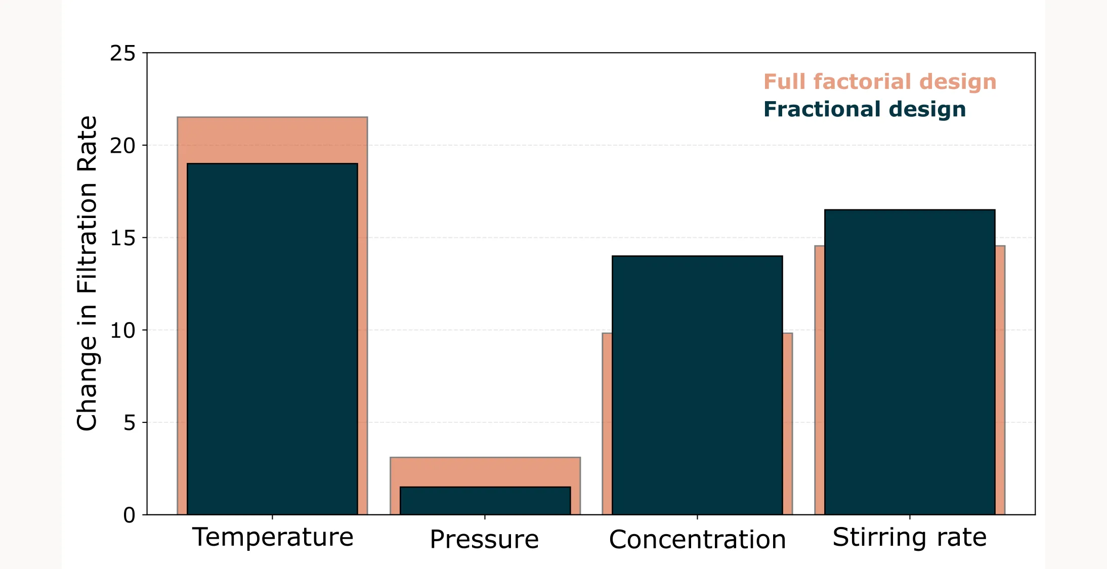
Repeating this for the other factors gives us a barplot similar to the one in the post A step by step example of a full factorial design. The results are consistent with the full factorial design, showing that Temperature has the strongest effect. However, the absolute values of the main effects differ slightly due to aliasing. The observed effect is a combination of the main effect and the aliased three-way interaction:

Observed Effect = T + P × CoF × RPM

Observed Effect = P + T × CoF × RPM

Observed Effect = CoF + T × P × RPM

Observed Effect = RPM + T × P × CoF

However, as we can see, the effect of the three-way interactions is rather small, almost negligible. So we can interpret the main effects in a Resolution IV design almost the same as main effects in a full factorial design.

Rule of thumb: The higher the order of the interaction, the less important they are, the lower their effect. Usually main effects and two-way interactions have practical relevance, and everything above (three-way; four-way; …) does not.

Visual Analysis: Two-Way Interactions

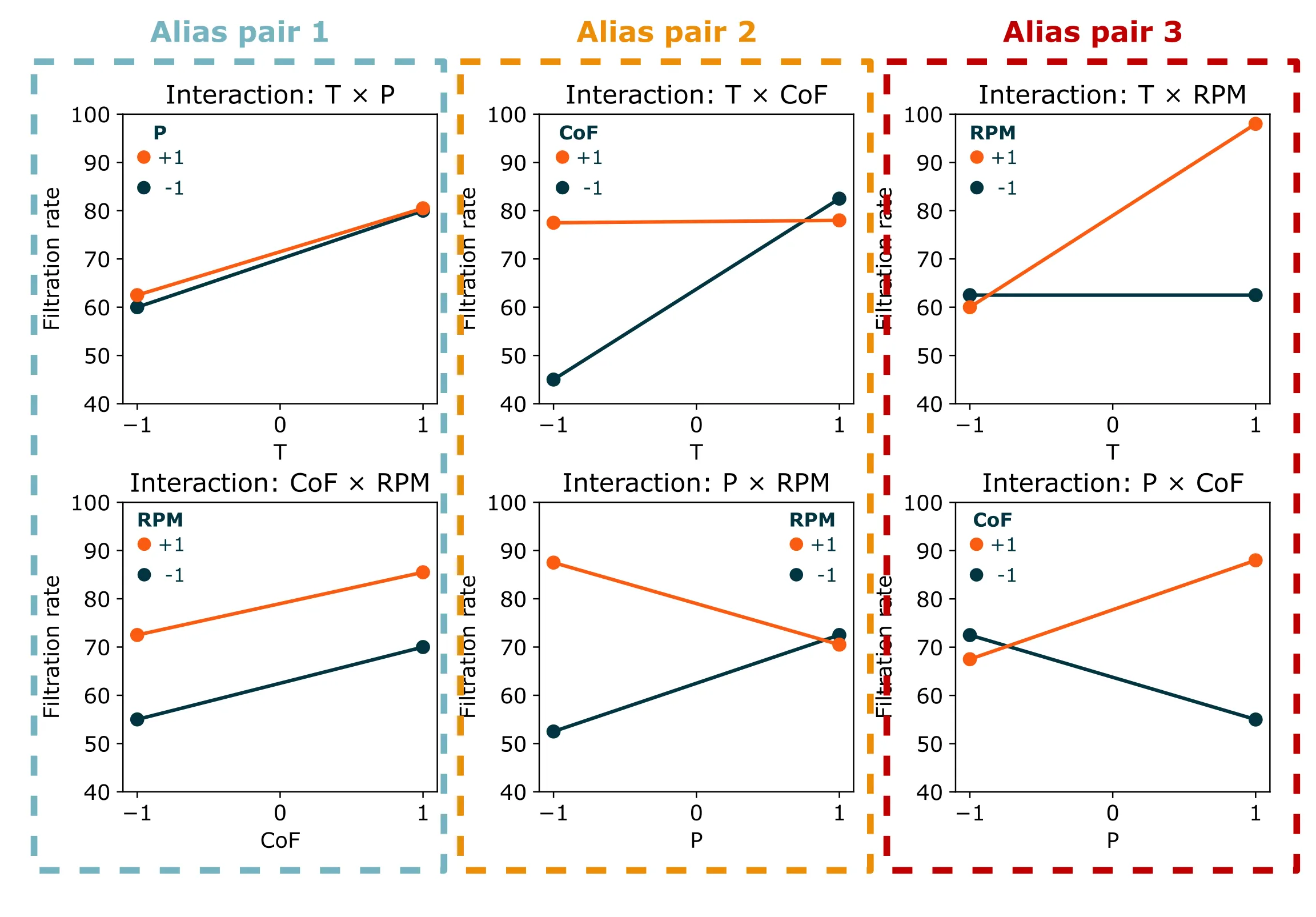
Two-way interactions are trickier in a Resolution IV design because they are aliased with each other, as we can see in the two-way interaction plots below.

Short reminder: Parallel lines indicate little or no interaction, meaning the factors work independently. Non-parallel or crossing lines suggest an interaction is present, where the factors influence each other.

From the full factorial data (see here) that we have in this case, we know that the T×CoF and T×RPM interactions are the important ones, and all others are more or less negligible. But let’s see if we could reach the same conclusion with the fractional design.

We notice no interaction in the first alias pair. Of course, it’s possible that both interactions are large but in opposite directions, because then they would cancel each other out. However, we shouldn’t overcomplicate things. Often the simplest solution is the correct one.

The interpretation of the second alias pair is more complicated. Here we see significant interactions, and due to aliasing we cannot tell if the interaction between T×CoF is large or between P×RPM. However, if we keep it simple, we can make an educated guess based on the main effects. Since Pressure has a negligible main effect, interactions involving Pressure are also likely insignificant. Therefore, the T×CoF interaction in the second alias pair is the important one, and we can neglect the P×RPM interaction.

The same applies to the third alias pair. We don’t know whether T×RPM is large or P×CoF is large. Both could also be medium. But again, since the pressure main effect is insignificant, we assume that T×RPM is the significant interaction and P×CoF is negligible.

And just like that, by carefully interpreting the data (using common sense and expert knowledge), we can extract meaningful insights even with fewer runs.

Key Takeaways

• Fractional factorial designs are a cost-effective way to explore multiple factors, especially in the screening phase.
• Confounding is a trade-off, but higher-order interactions are often negligible in practice. With common sense and expert knowledge, it is possible to make sense even of aliased data.
• Resolution is a measure of confounding severity. Resolution III designs should be used cautiously, Resolution IV designs are ideal for screening, and Resolution V designs are nearly as informative as full factorial designs.
• Fractional designs are best suited for early-stage experiments where the goal is to identify key factors.

Up next:

<< Create a Fractional Factorial Design in Python >>

<< Mathematical Models in DOE >>