Mathematical Models in DOE
We’ve explored full and fractional factorial designs, and so far, we’ve relied on data visualization using main effect and interaction plots to understand our system.
While data visualisation provides qualitative insights, quantifying these effects is important for more complex goals. Just imagine instead of just increase the filtration rate, we actually want to adjust the filtration rate for every different product we have in our portfolio, each requiring a slightly different optimal rate. Or maybe the process itself requires that we change the filtration rate over time. Like slow at the beginning, faster in the middle, then slower again toward the end.
This is where we need a mathematical equation that can predict the filtration rate based on any combination of input factors so that at any given time we know how to adjust the process settings to exactly achieve the filtration rate we need. We need a mathematical model.

What is a mathematical model?
A mathematical model is essentially a simplified representation of reality. It’s an equation that describes the relationship between your input factors (like temperature, concentration, stirring rate) and your response (like filtration rate). In general, we can write it as:
Response = f(Factors) + Error
It consists of three main parts:
Factors – the variables you control in your experiment, such as temperature, pressure, or concentration.
f(·) – the mathematical function that links those factors to the response. Depending on the situation, this could be a simple straight line, a polynomial, or something more complex. Important! The data you gather must fit the type of model you plan to use.
Error – the part of the response the model can’t explain. This includes measurement noise, random variation, or effects from factors you didn’t include.
Instead of saying “increase temperature to get a higher filtration rate,” a mathematical model tells you precisely: “increase temperature by 5°C and you’ll get exactly 12.5 units more filtration rate.” It transforms your qualitative understanding into something quantitative.
The beauty of a mathematical model is that it even lets you predict what will happen under conditions you haven’t tested yet. It can tell you what happens at 85°C when you’ve only tested 80°C and 90°C. But only if it is a good model.
Every Model is Wrong, But Some Are Useful
The statistician George Box famously said, “Every model is wrong, but some models are useful.” This highlights an important truth about mathematical modeling in DOE. Models are simplified representations of reality, and simplification inevitably means leaving something out.
However, that’s okay. Your model doesn’t need to explain every tiny fluctuation in your data. It just needs to capture the relationships that matter for your specific goals. Sometimes, a model that explains 85% of the variation is more useful than one that explains 95% but is twice as complicated and requires twice as many experiments.
Building Your First Model
Let’s revisit our filtration rate example and create our first mathematical model to predict the filtration rates we measured.
Note: The dataset here is coded at two levels per factor (−1 = low, +1 = high).
Predicting filtration rate from temperature
We’ll start simple and try to predict the filtration rates based only on temperature (coded factor T).
Looking at our experimental data, the regression analysis gives us the coefficients for our equation:
Filtration Rate = β₀ + β₁ × Temperature
Where:
- β₀ is the intercept (average filtration rate)
- β₁ is the slope (how much filtration rate changes per unit of temperature)
Note: In this case, the data we gathered only allows us to fit a linear model. For more complex models, we need to use more advanced designs, such as a central composite design.
From our regression analysis of the experimental data, we get:
Filtration Rate = 70.1 + 10.8 × T
This equation tells us that for every unit increase in temperature (coded variables!), the filtration rate increases by 10.8 units.
Now we can predict filtration rates for any temperature within our experimental range, not just the specific temperatures we tested.
How good are the predictions?
But how accurate is this model? Let’s use it to predict the filtration rates for the experimental design plan and compare them to the actual filtration rates we measured:
| Run | T | P | CoF | RPM | Filtration_rate | Predicted |
|---|---|---|---|---|---|---|
| 1.0 | -1.0 | -1.0 | -1.0 | -1.0 | 45.0 | 59.3 |
| 2.0 | 1.0 | -1.0 | -1.0 | -1.0 | 71.0 | 80.9 |
| 3.0 | -1.0 | 1.0 | -1.0 | -1.0 | 48.0 | 59.3 |
| 4.0 | 1.0 | 1.0 | -1.0 | -1.0 | 65.0 | 80.9 |
| 5.0 | -1.0 | -1.0 | 1.0 | -1.0 | 68.0 | 59.3 |
| 6.0 | 1.0 | -1.0 | 1.0 | -1.0 | 60.0 | 80.9 |
| 7.0 | -1.0 | 1.0 | 1.0 | -1.0 | 80.0 | 59.3 |
| 8.0 | 1.0 | 1.0 | 1.0 | -1.0 | 65.0 | 80.9 |
| … | … | … | … | … | … | … |
We see that the predictions aren’t very accurate, which makes sense since we only used one of the four factors in our model.
Adding more factors to our model
Let’s include the other factors to create a more comprehensive model. We’ll add all four main effects: temperature (T), pressure (P), concentration of formaldehyde (CoF), and stirring rate (RPM).
Our expanded model now looks like:
Filtration rate = 70.1 + 10.8×T + 1.6×P + 4.9×CoF + 7.3×RPM
This equation implies (per one coded unit change):
- Increasing T raises the filtration rate by about 10.8 units
- Increasing P raises it by about 1.6 units
- Increasing CoF raises it by about 4.9 units
- Increasing RPM raises it by about 7.3 units
Let’s see how this improved model performs:
| Run | T | P | CoF | RPM | Filtration_rate | Predicted |
|---|---|---|---|---|---|---|
| 1.0 | -1.0 | -1.0 | -1.0 | -1.0 | 45.0 | 45.4 |
| 2.0 | 1.0 | -1.0 | -1.0 | -1.0 | 71.0 | 67.1 |
| 3.0 | -1.0 | 1.0 | -1.0 | -1.0 | 48.0 | 48.6 |
| 4.0 | 1.0 | 1.0 | -1.0 | -1.0 | 65.0 | 70.2 |
| 5.0 | -1.0 | -1.0 | 1.0 | -1.0 | 68.0 | 55.3 |
| 6.0 | 1.0 | -1.0 | 1.0 | -1.0 | 60.0 | 76.9 |
| 7.0 | -1.0 | 1.0 | 1.0 | -1.0 | 80.0 | 58.4 |
| 8.0 | 1.0 | 1.0 | 1.0 | -1.0 | 65.0 | 80.1 |
| … | … | … | … | … | … | … |
The predictions are better for some runs, but we still have notable errors. This suggests we’re missing something important—the interactions between factors.
Including interactions
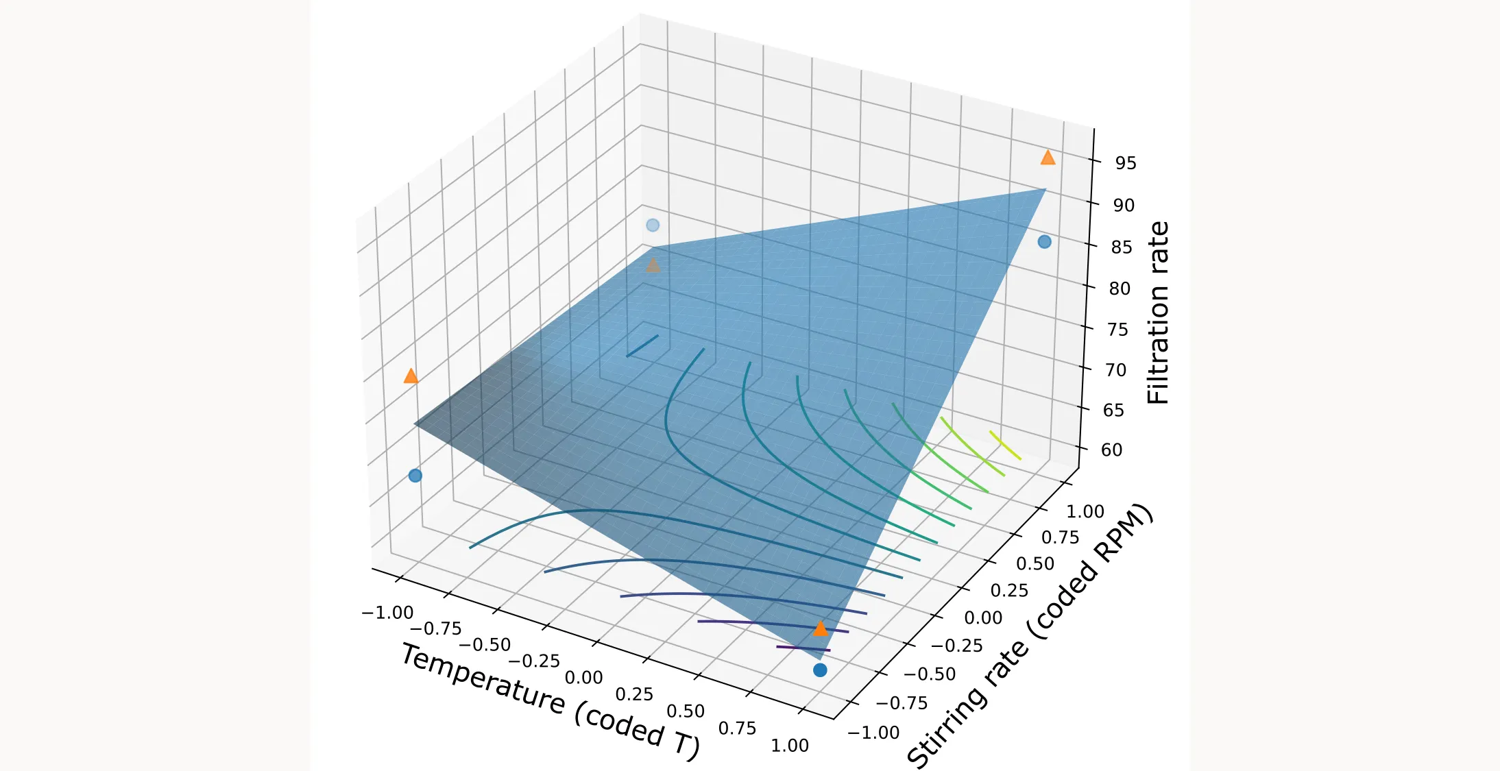
From our previous analysis through visualization we know that two interactions are particularly relevant: T × CoF and T × RPM. Remember, an interaction means the effect of one factor depends on the level of another factor.
Let’s add these interactions to our model:
Filtration rate = 70.1 + 10.8×T + 1.6×P + 4.9×CoF + 7.3×RPM - 9.1×T_CoF + 8.3×T_RPM
The interaction terms tell us:
- The T × CoF coefficient (-9.1) adjusts the temperature effect depending on the concentration level. It means that when both temperature and concentration are high, the effect is less than the sum of their individual effects.
- The T × RPM coefficient (8.3) adjusts the temperature effect depending on the stirring rate level. It means that when both temperature and stirring rate are high, the effect is greater than the sum of their individual effects.
Now let’s see how our predictions look with interactions included:
| Run | T | P | CoF | RPM | Filtration_rate | Predicted |
|---|---|---|---|---|---|---|
| 1.0 | -1.0 | -1.0 | -1.0 | -1.0 | 45.0 | 44.7 |
| 2.0 | 1.0 | -1.0 | -1.0 | -1.0 | 71.0 | 67.8 |
| 3.0 | -1.0 | 1.0 | -1.0 | -1.0 | 48.0 | 47.8 |
| 4.0 | 1.0 | 1.0 | -1.0 | -1.0 | 65.0 | 70.9 |
| 5.0 | -1.0 | -1.0 | 1.0 | -1.0 | 68.0 | 72.7 |
| 6.0 | 1.0 | -1.0 | 1.0 | -1.0 | 60.0 | 59.6 |
| 7.0 | -1.0 | 1.0 | 1.0 | -1.0 | 80.0 | 75.8 |
| 8.0 | 1.0 | 1.0 | 1.0 | -1.0 | 65.0 | 62.7 |
| … | … | … | … | … | … | … |
Great! Now our predictions are much more accurate. While the model isn’t perfect, it captures the essential relationships in our system and can reliably predict filtration rates for any combination of our factors within the experimental range.
Choosing What to Include
This brings us to a crucial question: which factors and interactions should we include in our model? Including everything might seem like the safest approach, but it can lead to overfitting—a model that perfectly describes your experimental data but fails miserably when predicting new conditions.
To avoid this, we only include the important factors. But how do we know which factors are important? We use a technique called Analysis of Variance (ANOVA). We’ll cover this in a future blog post.
Bringing It All Together
Mathematical models let you move beyond general observations like “temperature up, rate goes up” and instead provide precise equations for planning and control. The key is balance: keep models simple enough to be practical but detailed enough to meet your goals.
Our full factorial example gave us a linear model that works well within the tested range. If you notice systematic errors or suspect curved behavior, that’s your signal to try more advanced designs like central composite designs. These allow you to model curvature and capture a more complete picture of your system.
Modeling is an iterative process. Start simple, test your predictions, refine where needed, and always let your experimental goals guide the level of complexity.