How to perform ANOVA
In our last blog post, we learned what a model is and what it can do for us. We even built one for our filtration rate experiment. But if you’re being honest, the process felt a bit random how we added the model parameters didn’t it?
There’s actually a systematic, statistically rigorous method for building models in DoE, and it’s called ANOVA (Analysis of Variance). ANOVA helps us answer a fundamental question: “Which parameters actually matter, and which ones are just noise?”
Think of ANOVA as your quality control inspector. It looks at every potential parameter—main effects, interactions, quadratic terms—and gives each one a pass/fail grade. Pass means “this parameter is contributing real information to your model.” Fail means “this parameter is just adding complexity without value.”
The Basic Concept of ANOVA
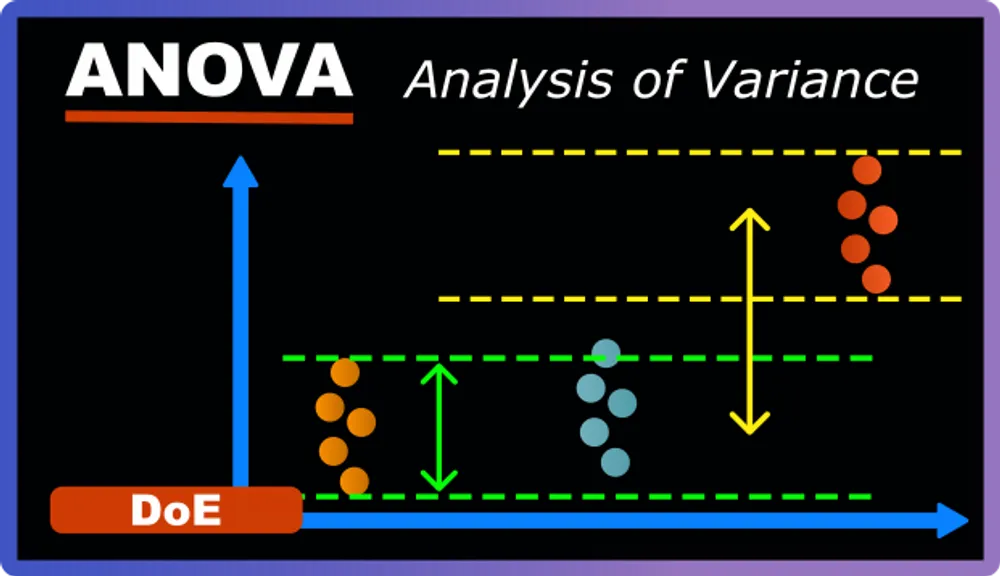
ANOVA works by comparing two types of variation in your data:
Within-group variance: How much do measurements vary when you keep a factor at the same level? This represents your measurement error, experimental noise, and all the uncontrolled factors you can’t account for.
Between-group variance: How much do your measurements change when you actually change your factor level? This represents the real effect of your factors.
If changing a factor creates more variation than your measurement noise, that factor significantly affects your response. If the variation from changing the factor is about the same as your measurement noise, that factor probably isn’t doing much.
Here’s a concrete example from our filtration rate experiment:
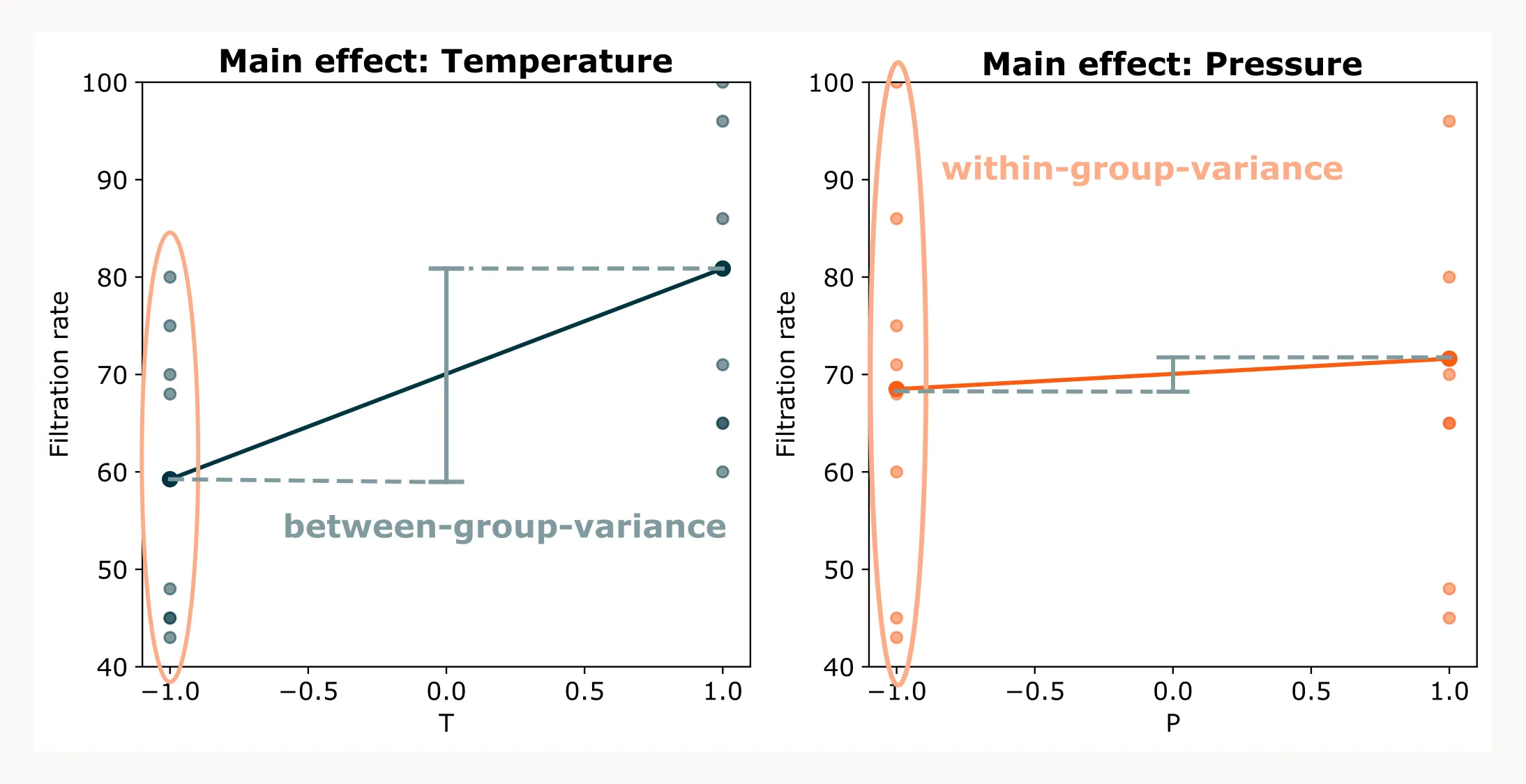
The plot above illustrates the main effect of temperature (left) and pressure (right). Remember, main effects are calculated as averages: all filtration rates measured at the low level (-1) of a factor are averaged, and the same is done for the high level (+1). These averages are then plotted to show the overall effect of increasing the factor.
In other words, the slope of each line tells us: “On average, if we increase temperature (or pressure) from -1 to +1, the filtration rate changes by this much.” Each average, however, comes from a group of individual measurements. ANOVA compares the variation within each group (measurements at the same factor level) to the variation between the group means (the difference from -1 to +1).
When we compare the two plots, the effect of temperature stands out more clearly than that of pressure. Changing the temperature leads to a noticeable shift in the average filtration rate. The spread within each group is noticeable, but it seems that temperature does have a significant effect on filtration rate. For pressure, the variation within groups is much larger than the between-group variation (which is hardly there). Therefore, it seems that the main effect of temperature is significant, while pressure is not.
What Makes a Parameter Significant?
This is the basic concept of ANOVA, but simply looking at the data as we did above can be subjective. You might come to a different conclusion than I did. There has to be a better way, right? Yes!
A parameter is considered statistically significant when the variation it causes in your response is substantially larger than what you’d expect from random noise alone. We quantify this using the so-called p-value.
The p-value tells you the probability that you’d see this large an effect even if the parameter actually had no real impact. Think of it as asking: “If this factor truly doesn’t matter, what’s the chance I’d still see this big a change in my results just by random luck?”
- Low p-value (typically < 0.05): Very unlikely this effect happened by chance. The parameter is probably significant.
- High p-value (> 0.05): This effect likely happened by chance and could be easily explained by random variation. The parameter is probably not significant.
The 0.05 threshold means we’re accepting a 5% chance of being wrong—that is, a 5% chance that we’ll conclude a parameter is significant when it actually isn’t. Most of the time, we’re comfortable with this level of risk, but you can be more conservative (use 0.01 for a 1% chance) or more liberal (use 0.10 for a 10% chance) depending on your situation.
Note: Significant doesn’t always mean relevant. A parameter might have a statistically significant effect but such a tiny practical impact that it’s not worth worrying about. Always consider both statistical significance and practical importance in combination.
How to Perform ANOVA
Choosing the Right Software
First things first: What software do you need to perform ANOVA?
You’ll need some kind of statistics software. There are plenty of choices for all kinds of budgets:
- Commercial software: JMP, Minitab, Design Expert, and MODDE are industry standards. They’re powerful and offer much more functionality than just ANOVA. The drawback is their cost, which can be worth it but might not fit every budget.
- Budget-friendly option: I personally like and recommend Datatab for its simplicity and affordability. It handles most DoE analyses without the complexity of bigger packages.
- Free option: Programming languages like Python or R can handle ANOVA perfectly well. They’re versatile and offer limitless functionality. The only drawback is that you need to be somewhat familiar with programming. But here’s a pro tip: with AI evolving, it’s easier than ever to get started. In fact, you can already do it in tools like ChatGPT without needing to learn a programming language. However, if you want to keep control over your data, I’ve made a tutorial on performing ANOVA with Python here.
No matter which software you choose, the workflow is more or less the same.
The Basic Workflow
- Build your initial model: Start with a mathematical model that includes all the parameters you want to test (main effects, interactions, quadratic terms, etc.).
- Run the ANOVA: Your software calculates the statistical significance of each parameter and presents the results in an ANOVA table.
- Examine the p-values: Look at each parameter’s p-value in the ANOVA table.
- Make decisions: Keep parameters with p-values below your significance threshold (typically 0.05), and eliminate those above it.
- Repeat if necessary: Remove non-significant parameters and re-run the analysis until all p-values are below your threshold. This is your final model.
This process involves some trial and error, but there are two more systematic approaches I recommend.
Systematic Approaches to Testing Parameters
You have two main approaches for building your model:
Approach 1: Backward Elimination
Start with everything—all main effects, all interactions, even higher-order terms if you have them. Then systematically remove the weakest performers:
- Run ANOVA on the full model.
- Identify the parameter with the highest p-value (least significant).
- Remove that parameter and refit the model.
- Repeat until only significant parameters remain.
This approach ensures you don’t accidentally miss important effects. It’s like starting with a fully loaded toolbox and gradually removing the tools you don’t actually need.
Approach 2: Forward Selection
Start with just the main effects, then add parameters you think might be significant:
- Begin with a simple model (main effects only).
- Test adding remaining parameters individually.
- Keep them if they meet your significance criteria; drop them if they don’t.
- Repeat until no additional parameters meet your significance criteria.
Visualizing your results often gives you a good idea of which effects and interactions might be significant. Use ANOVA to confirm your intuition.
Example: Filtration Rate Model Building
Let’s apply both approaches to our filtration rate example with Temperature (T), Pressure (P), Formaldehyde concentration (CoF), and Stirring rate (RPM).
Backward Elimination Example
Step 1: Start with the full model including all main effects and interactions:
ANOVA Results (Initial):
| Source | DF | Sum of Squares | Mean Square | F-ratio | p-value |
|---|---|---|---|---|---|
| T | 1 | 1871 | 1871 | 247.3 | 0.040 |
| P | 1 | 39 | 39 | 5.17 | 0.264 |
| T:P | 1 | 0.06 | 0.06 | 0.01 | 0.942 |
| CoF | 1 | 390 | 390 | 51.6 | 0.088 |
| T:CoF | 1 | 1314 | 1314 | 173.8 | 0.048 |
| P:CoF | 1 | 22.6 | 22.6 | 2.98 | 0.334 |
| T:P:CoF | 1 | 14.1 | 14.1 | 1.86 | 0.403 |
| RPM | 1 | 856 | 856 | 113.1 | 0.060 |
| T:RPM | 1 | 1106 | 1106 | 146.2 | 0.053 |
| P:RPM | 1 | 0.56 | 0.56 | 0.07 | 0.830 |
| T:P:RPM | 1 | 68.1 | 68.1 | 9.00 | 0.205 |
| CoF:RPM | 1 | 5.06 | 5.06 | 0.67 | 0.563 |
| P:CoF:RPM | 1 | 27.6 | 27.6 | 3.64 | 0.307 |
| Residual | 1 | 7.56 | 7.56 | NaN | NaN |
If you are not sure about how to read an ANOVA table, take a look at this blog post: Understanding the ANOVA Table Output
Step 2: Work from the highest order interactions down to the lowest. At each step, remove the term with the highest p-value. In this case, we first remove the three-way interaction T×CoF×RPM since it has the highest p-value out of all the three way interactions. Then refit the model and repeat.
ANOVA Results (2nd step):
| Source | DF | Sum of Squares | Mean Square | F-ratio | p-value |
|---|---|---|---|---|---|
| T | 1 | 1871 | 1871 | 206.4 | 0.005 |
| P | 1 | 39 | 39 | 4.3 | 0.174 |
| T:P | 1 | 0.06 | 0.06 | 0.01 | 0.941 |
| CoF | 1 | 390 | 390 | 43.0 | 0.023 |
| T:CoF | 1 | 1314 | 1314 | 145.0 | 0.007 |
| P:CoF | 1 | 22.6 | 22.6 | 2.5 | 0.255 |
| RPM | 1 | 856 | 856 | 94.4 | 0.010 |
| T:RPM | 1 | 1106 | 1106 | 122.0 | 0.008 |
| P:RPM | 1 | 0.56 | 0.56 | 0.06 | 0.827 |
| T:P:RPM | 1 | 68.1 | 68.1 | 7.5 | 0.111 |
| CoF:RPM | 1 | 5.06 | 5.06 | 0.56 | 0.533 |
| P:CoF:RPM | 1 | 27.6 | 27.6 | 3.0 | 0.223 |
| Residual | 2 | 18.1 | 9.1 | NaN | NaN |
Step 3: Continue removing non-significant terms (P, RPM, and other interactions) until only significant parameters are left.
ANOVA Results (final):
| Source | DF | Sum of Squares | Mean Square | F-ratio | p-value |
|---|---|---|---|---|---|
| T | 1 | 1871 | 1871 | 95.9 | < 0.001 |
| CoF | 1 | 390 | 390 | 20.0 | 0.001 |
| RPM | 1 | 856 | 856 | 43.8 | < 0.001 |
| T:CoF | 1 | 1314 | 1314 | 67.3 | < 0.001 |
| T:RPM | 1 | 1106 | 1106 | 56.7 | < 0.001 |
| Residual | 10 | 195 | 19.5 | NaN | NaN |
This is your final model with an R2 of 0.97:
Filtration Rate = 70.1 + 10.8·T + 4.9·CoF + 7.3·RPM − 9.1·(T×CoF) + 8.3·(T×RPM)`
Forward Selection Example
Step 1: Start with main effects only:
ANOVA Results (Initial):
| Source | DF | Sum of Squares | Mean Square | F-ratio | p-value |
|---|---|---|---|---|---|
| T | 1 | 1871 | 1871 | 8.0 | 0.017 |
| P | 1 | 39 | 39 | 0.17 | 0.691 |
| CoF | 1 | 390 | 390 | 1.7 | 0.223 |
| RPM | 1 | 856 | 856 | 3.7 | 0.082 |
| Residual | 11 | 2576 | 234 | NaN | NaN |
Step 2: Test adding interactions. Start with those that the visualization suggested that are significant. In this case that was T×CoF and TxRPM.
ANOVA Results (2nd step):
| Source | DF | Sum of Squares | Mean Square | F-ratio | p-value |
|---|---|---|---|---|---|
| T | 1 | 1871 | 1871 | 107.9 | < 0.001 |
| P | 1 | 39 | 39 | 2.3 | 0.168 |
| CoF | 1 | 390 | 390 | 22.5 | 0.001 |
| RPM | 1 | 856 | 856 | 49.3 | < 0.001 |
| T:CoF | 1 | 1314 | 1314 | 75.8 | < 0.001 |
| T:RPM | 1 | 1106 | 1106 | 63.8 | < 0.001 |
| Residual | 9 | 156 | 17.3 | NaN | NaN |
Step 3: Add other interactions that you think could be significant. For example also the three way interaction between TxCoFxRPM.
ANOVA Results (3rd step):
| Source | DF | Sum of Squares | Mean Square | F-ratio | p-value |
|---|---|---|---|---|---|
| T | 1 | 1871 | 1871 | 102.8 | < 0.001 |
| P | 1 | 39 | 39 | 2.1 | 0.181 |
| CoF | 1 | 390 | 390 | 21.4 | 0.00169 |
| RPM | 1 | 856 | 856 | 47.0 | < 0.001 |
| T:CoF | 1 | 1314 | 1314 | 72.3 | < 0.001 |
| T:RPM | 1 | 1106 | 1106 | 60.8 | < 0.001 |
| T:CoF:RPM | 1 | 10.6 | 10.6 | 0.6 | 0.468 |
| Residual | 8 | 145.5 | 18.2 | NaN | NaN |
But as we see, we find no other significant interactions and we can even remove the main effect of pressure as it also has a p-value that is higher than our threshold. So we conclude the final model is the same as with the backward elimination approach:
Filtration Rate = 70.1 + 10.8·T + 4.9·CoF + 7.3·RPM − 9.1·(T×CoF) + 8.3·(T×RPM)
The Final Model: Summary and Conclusion
Our final model gives us a clean, statistically justified equation for predicting filtration rate. Every parameter in the model has earned its place through rigorous statistical testing.
Let’s compare how well our streamlined model performs against a model that includes all the original parameters:
Statistical Model (only significant parameters):
Filtration Rate = 70.1 + 10.8·T + 4.9·CoF + 7.3·RPM − 9.1·(T×CoF) + 8.3·(T×RPM)
Full Model (all parameters):
Filtration Rate = 70.1 + 10.8·T + 1.6·P + 0.1·(T×P) + 4.9·CoF − 9.1·(T×CoF) + 1.2·(P×CoF) + 0.9·(T×P×CoF) + 7.3·RPM + 8.3·(T×RPM) − 0.2·(P×RPM)
| T | P | CoF | RPM | Measured | Full model | Only significant params |
|---|---|---|---|---|---|---|
| -1 | -1 | -1 | -1 | 45 | 44 | 46 |
| 1 | -1 | -1 | -1 | 71 | 72 | 67 |
| -1 | 1 | -1 | -1 | 48 | 49 | 49 |
| 1 | 1 | -1 | -1 | 65 | 64 | 70 |
| -1 | -1 | 1 | -1 | 68 | 69 | 72 |
| 1 | -1 | 1 | -1 | 60 | 59 | 60 |
| -1 | 1 | 1 | -1 | 80 | 79 | 75 |
| 1 | 1 | 1 | -1 | 65 | 66 | 64 |
| -1 | -1 | -1 | 1 | 43 | 44 | 42 |
| 1 | -1 | -1 | 1 | 100 | 99 | 100 |
| -1 | 1 | -1 | 1 | 45 | 44 | 45 |
| 1 | 1 | -1 | 1 | 104 | 105 | 103 |
| -1 | -1 | 1 | 1 | 75 | 74 | 72 |
| 1 | -1 | 1 | 1 | 86 | 87 | 90 |
| -1 | 1 | 1 | 1 | 70 | 71 | 75 |
| 1 | 1 | 1 | 1 | 96 | 95 | 93 |
The full model provides slightly more accurate predictions, but it’s likely not general and risks overfitting. It might perform worse on new data.
A Critical Caveat: ANOVA Assumptions
Before you rush to apply these steps to your dataset, there’s an important disclaimer: ANOVA only gives reliable results when certain assumptions are met. These assumptions are the foundation of the entire statistical analysis. If they’re violated, your p-values and conclusions can be wrong.
These assumptions are:
- Normality: Your residuals (prediction errors) should follow a normal distribution.
- Independence: Each measurement should be independent of the others.
- Equal variance: The scatter in your data should be consistent across all conditions.
Getting these assumptions right is just as important as running ANOVA itself. Therefore we cover them thoroughly in the next blog post.