In our last blog post, we used ANOVA to systematically build a mathematical model for our filtration rate experiment. We identified which parameters were significant, eliminated the noise, and ended up with a clean, predictive model.

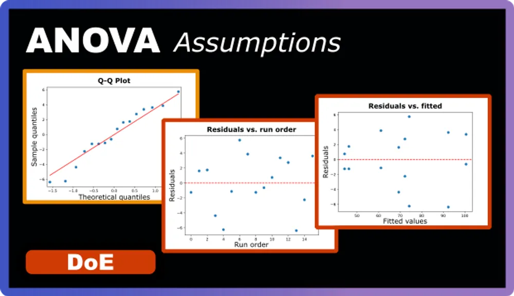
But we glossed over something important: all those p-values, F-ratios, and statistical conclusions we relied on are only valid if our data meets certain fundamental requirements. These are called ANOVA assumptions, and there are three you always need to check:

1. Independence: Each observation should be independent of all others
2. Normality: The residuals should follow a normal distribution
3. Equal Variance (Homoscedasticity): The variability should be consistent across all conditions

They’re like the foundation of a house—you can build a beautiful structure on top, but if the foundation isn’t solid, the whole thing becomes unreliable.

How to Check These Assumptions

Here’s the practical workflow:

1. Run your ANOVA. Build your model, get your p-values, and see which effects are significant.
2. Check the assumptions. Use the model’s residuals and fitted values to diagnose independence, normality, and equal variance.
3. If assumptions are violated, adjust and repeat. This might mean transforming your data, tweaking your model (like adding certain interactions back in), or improving your experimental design to allow for quadratic model terms. Then, re-run the ANOVA and check again.

You might wonder: if assumptions are so important, why not check them before running ANOVA? The answer is simple—most assumption checks require the model’s residuals and fitted values, which only exist after you’ve run the analysis. It’s similar to quality control in manufacturing: you don’t test the product before you make it; you make it and then test whether it meets specifications. If it fails, you adjust your process and try again.

With that in mind, let’s walk through each assumption and how to check it in practice.

Assumption 1: Independence

What it means: Each experimental run should be independent of all other runs. The result of run #1 shouldn’t influence the result of run #2, and so on.

Why it matters: If your observations are correlated, your apparent sample size is effectively smaller than what you think. This leads to overconfident p-values—you might conclude effects are significant when they’re actually just due to hidden patterns in your data.

Checking Independence

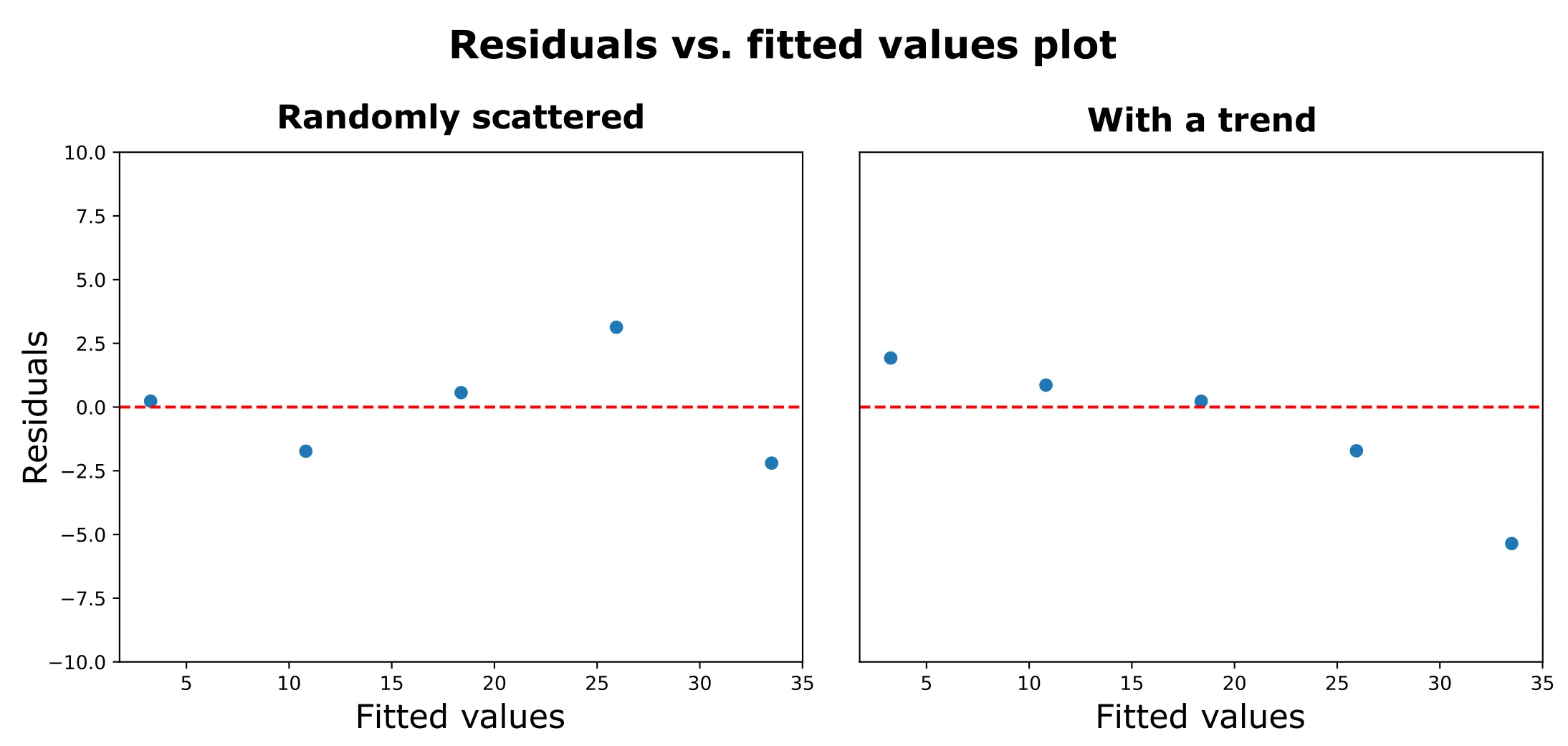
One of the best ways to check independence is to plot your residuals (the differences between observed and predicted values) in the order the experiments were run. This is called a “residuals vs. run order” plot.

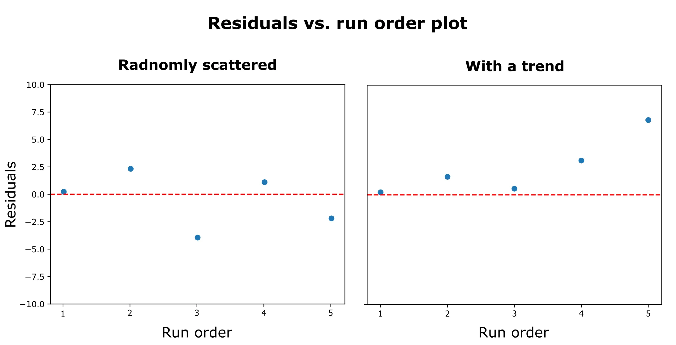
• Good Example: On the left, the residuals are randomly scattered around zero with no visible pattern. Each run appears independent—exactly what we want to see.
• Bad Example: On the right, the residuals show a clear downward trend, suggesting a time-dependent effect like equipment drift.

What to look for:

• Random scatter around zero: ✅ Independence assumption met
• Trends or patterns: ❌ Possible time-related effects
• Cycles: ❌ Systematic variation over time
• Increasing/decreasing variance: ❌ Equipment drift or learning effects

Common violations:

• Time trends: Equipment warming up, operator learning, material degradation
• Carryover effects: Previous experimental conditions affecting current results
• Measurement drift: Instruments becoming less accurate over time

Note: If your experimental design was properly randomized, this assumption is usually met. Problems typically arise from inadequate randomization or systematic changes during the experiment.

Our Filtration Rate Example

Let’s check independence for our experimental design:

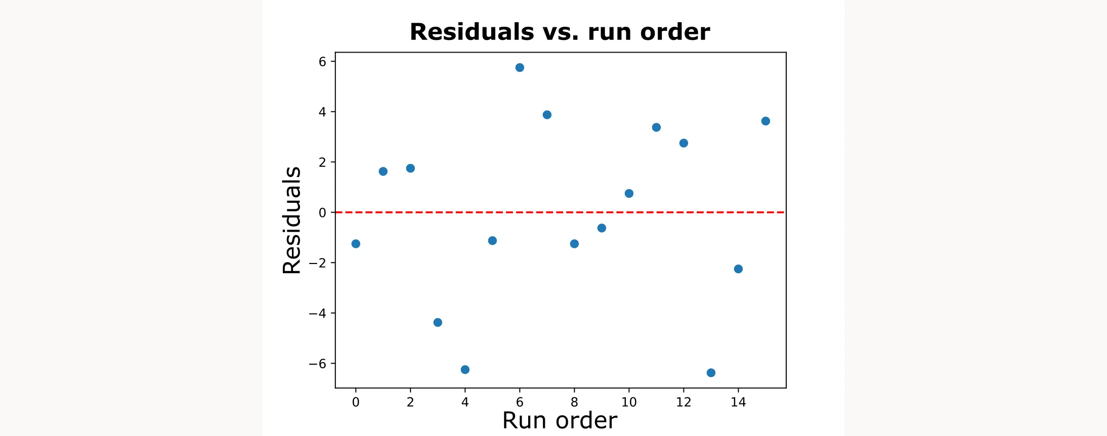
For our filtration rate experiment, I plotted the residuals in run order. The points bounce randomly around zero with no obvious trends or cycles, suggesting our runs were independent—no hidden time effects or equipment drift.

Assumption 2: Normality of Residuals

What it means: The residuals (differences between observed and predicted values) should follow a normal distribution.

Why it matters: ANOVA’s p-values are calculated assuming normal distributions. If your residuals are severely non-normal, your p-values can be wrong, leading to false conclusions about significance.

Checking Normality

The best way to check normality is with a normal probability plot (Q-Q plot). This plots your residuals against what they would be if they were perfectly normal. If the assumption holds, the points should fall roughly on a straight line in the Q-Q plot.

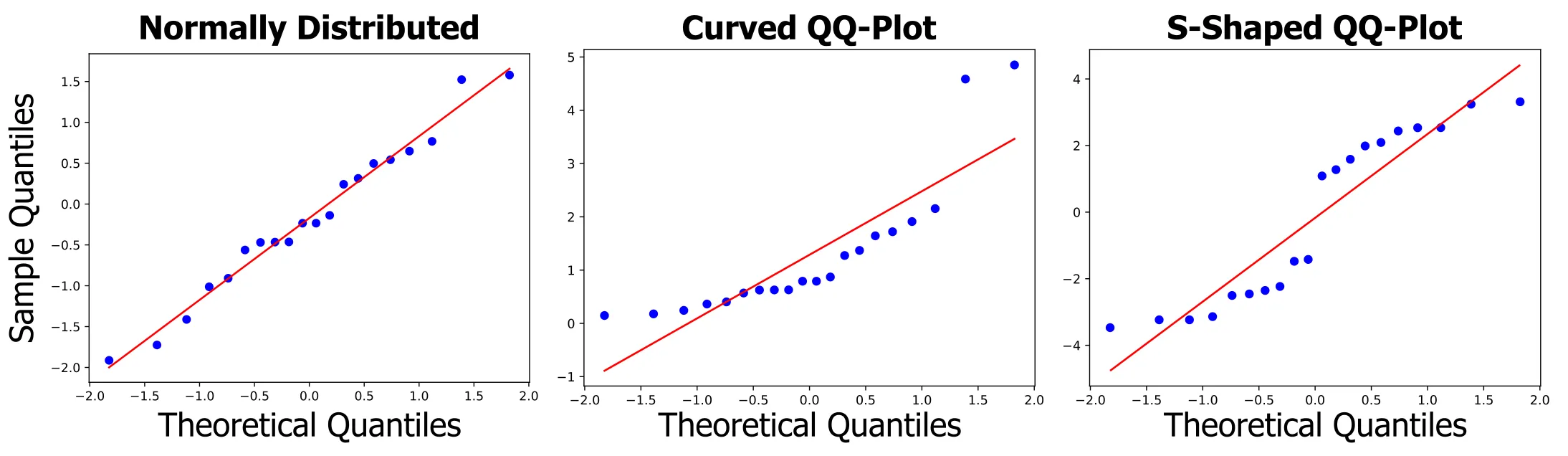
When residuals are normally distributed, the points should roughly follow the diagonal line.

What to look for:

• Points following the line closely: ✅ Normality assumption met
• Points deviating at the ends: ❌ Heavy or light tails
• S-shaped curves: ❌ Skewed data

Common violations:

• Heavy tails: More extreme values than expected under normality (outliers)
• Skewness: Residuals are not symmetric, often due to a transformation being needed

Solutions for normality violations:

• Data transformation: Log, square root, or Box–Cox transformations can often fix skewness and stabilize variance
• Outlier investigation: Check if extreme residuals represent measurement errors or unusual conditions
• Non-parametric alternatives: Use Kruskal-Wallis test instead of ANOVA if transformation doesn’t help

Our Filtration Rate Example

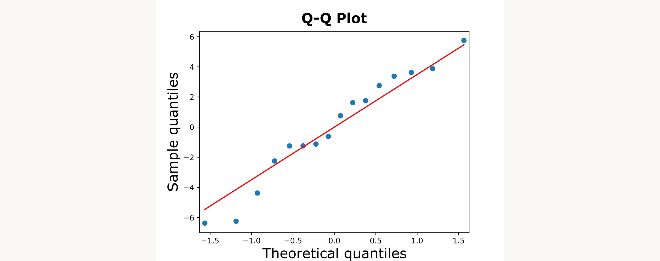
The figure shows a tiny S-shape, which is acceptable. Given the small deviation and balanced design, our ANOVA should be robust.

Assumption 3: Equal Variance (Homoscedasticity)

What it means: The variability in your response should be consistent across all experimental conditions. The scatter around your predicted values should be roughly the same everywhere.

Why it matters: ANOVA pools variance estimates across all conditions. If some conditions are much more variable than others, this pooling becomes inappropriate and can lead to incorrect conclusions.

Checking Equal Variance

The standard diagnostic is a plot of residuals versus fitted values. When equal variance holds, you should see random scatter with roughly constant spread across all fitted values.

What to look for:

• Random scatter with constant spread: ✅ Equal variance assumption met
• Funnel shape (wider spread at higher fitted values): ❌ Variance increases with the mean
• Inverted funnel (wider at low fitted values): ❌ Variance decreases with the mean
• Any systematic change in spread: ❌ Indicates heteroscedasticity (unequal variance)

If equal variance is violated:

• Try transforming your data (log, square root, or Box–Cox)
• Revisit the model (missing predictors/interactions) or the experimental design

Our Filtration Rate Example - Good Case

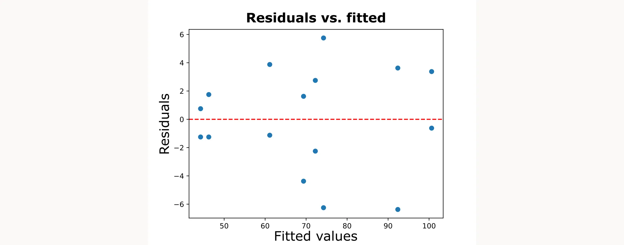
For our filtration rate example, the residuals vs. predicted plot looks good. The random scatter is exactly what we want to see.

The Bottom Line on ANOVA Assumptions

Every statistical test comes with assumptions. ANOVA’s assumptions are actually quite reasonable for most engineering and scientific applications. When violations occur, they’re usually fixable with straightforward modifications to your analysis approach.

Here’s what matters: check your assumptions, understand their impact, and make sure your analysis is reliable.

What’s Next?

If you want to learn how to perform ANOVA and check ANOVA assumptions, take a look at this blog post.

If you want to learn about central composite design (CCD) that lets you model curved relationships, take a look at this blog post.

Up next:

<< ANOVA in Python >>

<< A step by step example of a full factorial design >>