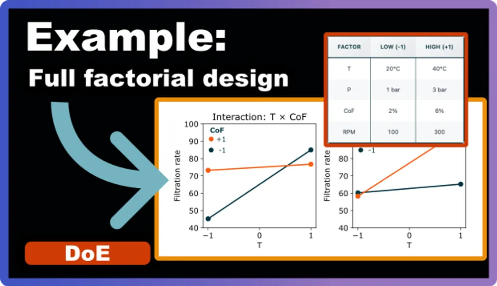
A step by step example of a full factorial design
Design of Experiments (DoE) can seem intimidating with its statistical terminology and complex analysis methods. But at its core, DoE is about systematically varying factors to understand their effects on your process or product.
Full factorial design is the simplest entry point into Design of Experiments (DoE). In this post, we’ll walk through a concrete example step by step. You’ll see how such a design is set up, what the results look like, and most importantly, how to interpret the results. For now, we skip the statistics part though and focus on just visuals and their interpretation.
What is a full factorial design?
A full factorial design tests every possible combination of the selected factors and their levels. The total number of runs is simply the product of the number of levels for each factor. With 4 factors each at 3 levels, you need 3×3×3×3 = 3^4 = 81 runs; already a sizable effort. Because the count grows exponentially, people often start with only two levels per factor (a 2^k design). When you need more than two levels (to detect curvature or optimize), you switch to more efficient response-surface designs (e.g. central composite or Box–Behnken). We’ll cover those later in our next blog post.
Example: filtration rate (2⁴ design)
In this study, we test how different settings influence filtration rate in an industrial process. We vary four factors we expect to matter:
- T – Temperature (°C)
- P – Pressure (bar)
- CoF – Concentration of formaldehyde (%)
- RPM – Agitation speed (revolutions per minute)
For each factor, we choose a practical operating range based on equipment limitations, safety considerations, and prior process knowledge:
- Temperature: 20–40°C
- Pressure: 1–3 bar
- Concentration: 2–6%
- RPM: 100–300
Using coded levels
To keep factors comparable and simplify analysis, we use coded levels rather than raw units: −1 for the lower setting and +1 for the higher setting. This standardization:
- Makes patterns easier to identify
- Ensures all factors have equal weight in the analysis
- Simplifies mathematical modeling
| Factor | Low (-1) | High (+1) |
|---|---|---|
| T | 20°C | 40°C |
| P | 1 bar | 3 bar |
| CoF | 2% | 6% |
| RPM | 100 | 300 |
Setting up the design plan
For our two-level full factorial design with four factors, we need to test every possible combination of low (−1) and high (+1) settings. This gives us 2×2×2×2 = 2⁴ = 16 experimental runs. The complete design table looks like this (measured filtration rate data already added):
| Run | T | P | CoF | RPM | Filtration Rate |
|---|---|---|---|---|---|
| 1 | −1 | −1 | −1 | −1 | 45 |
| 2 | −1 | −1 | −1 | +1 | 48 |
| 3 | −1 | −1 | +1 | −1 | 68 |
| 4 | −1 | −1 | +1 | +1 | 80 |
| 5 | −1 | +1 | −1 | −1 | 43 |
| 6 | −1 | +1 | −1 | +1 | 45 |
| 7 | −1 | +1 | +1 | −1 | 75 |
| 8 | −1 | +1 | +1 | +1 | 70 |
| 9 | +1 | −1 | −1 | −1 | 71 |
| 10 | +1 | −1 | −1 | +1 | 65 |
| 11 | +1 | −1 | +1 | −1 | 60 |
| 12 | +1 | −1 | +1 | +1 | 65 |
| 13 | +1 | +1 | −1 | −1 | 100 |
| 14 | +1 | +1 | −1 | +1 | 104 |
| 15 | +1 | +1 | +1 | −1 | 86 |
| 16 | +1 | +1 | +1 | +1 | 96 |
Important: In practice, you would run these experiments in random order to minimize the effects of uncontrolled variables (like ambient conditions, operator differences, or equipment drift over time). Most DoE software automatically randomizes the run order. In addition to that you would add replicate runs to account for experimental error. Blocking could be an option if for example the experiments are run on different machines or performed on different days.
Each row represents one experimental run with a unique combination of factor settings. For instance, Run 1 tests all factors at their low levels, while Run 16 tests all factors at their high levels.
Note: Design plans like this are typically created using dedicated DoE software, some of which can be quite expensive. However, you can easily create full factorial design plans using Python for free. Here’s a link to a short tutorial: Create a full factorial plan in Python.
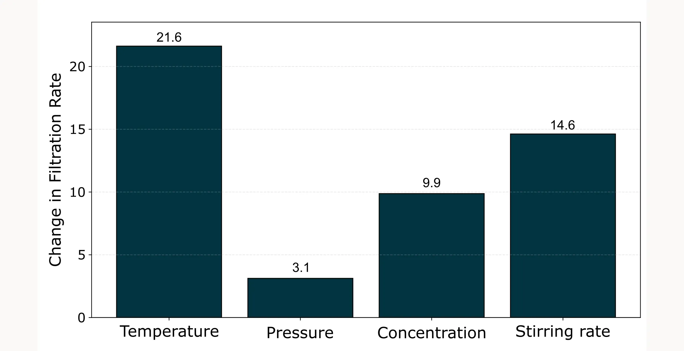
Visual analysis: main effects
After creating the design plan, you would go to the lab and run all 16 experiments according to the table above. Once you have collected the filtration rate data for each experimental run, it’s time to analyze the results.
The first step is to examine the main effects. A main effect describes the average impact each factor has on the filtration rate. In other words, it quantifies how much the response changes, on average, when a factor moves from its low level (−1) to its high level (+1).
Example calculation for Temperature (T): To find the main effect of Temperature, we:
- Average all runs where T = −1: (45 + 48 + 68 + 80 + 43 + 45 + 75 + 70) ÷ 8 = 59.3
- Average all runs where T = +1: (71 + 65 + 60 + 65 + 100 + 104 + 86 + 96) ÷ 8 = 80.9
- Calculate the difference: 80.9 − 59.3 = +21.6
This means that, on average, increasing Temperature from low to high increases the filtration rate by 21.6 units.
By repeating this calculation for all four factors and creating a barplot from the results (Figure 1), we can easily identify which factors have the strongest influence on filtration rate and which have lesser effects and we find that on average, an increase in temperature seems to increase the filtration rate the most while increasing the pressure doesn’t change the filtration rate much. Both of the other factors are somewhere in between.
Initial hypothesis: Based on these main effects alone, we might expect that setting all factors to their high levels (+1) would give us the maximum filtration rate.
But as we see in the table below, that is not quite true. In fact, the highest filtration rate is reached when the Concentration of Formaldehyde (CoF) is set to the low level and all other remaining factors are kept at high. So why is that?
| Setting | T | P | CoF | RPM | Filtration_rate |
|---|---|---|---|---|---|
| All parameters high | +1 | +1 | +1 | +1 | 96 |
| Actual maximum found | +1 | +1 | −1 | +1 | 104 |
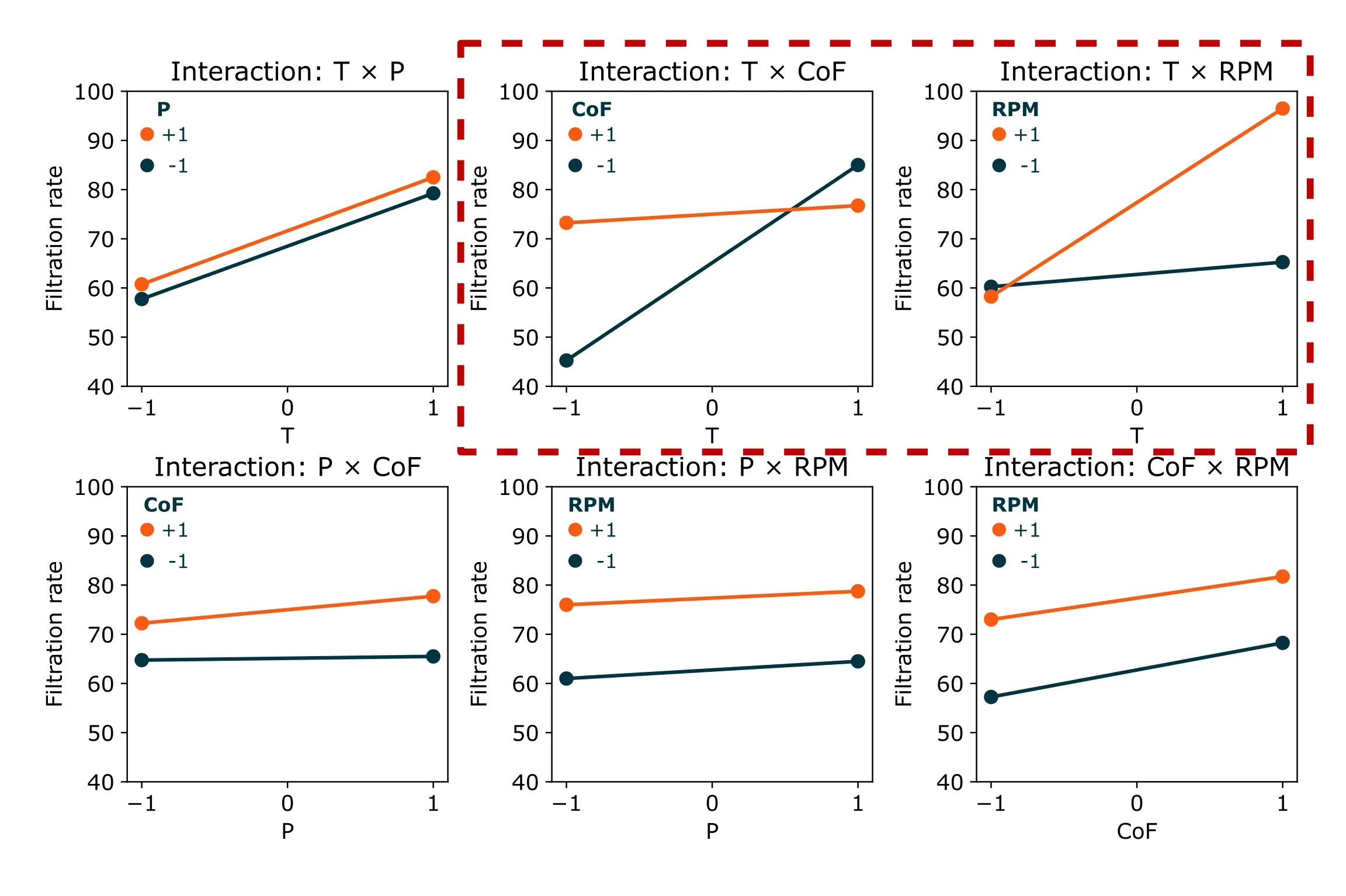
Visual analysis: two-way interactions
The answer lies in interactions between factors. Main effects tell us only the average impact of each factor across all conditions. But sometimes, factors don’t work independently. Instead, the effect of one factor depends on the level of another factor. This is called a two-way interaction.
The best way to spot interactions is through interaction plots:
How to read interaction plots:
- x-axis: levels of factor A (−1, +1)
- y-axis: mean response variable (filtration rate)
- two lines: one for each level of factor B (−1 vs +1)
Parallel lines ⇒ little/no interaction (factors work independently)
Non-parallel or crossing lines ⇒ interaction present (factors influence each other)
With four factors, we have six possible two-way interactions: T×P, T×CoF, T×RPM, P×CoF, P×RPM, CoF×RPM. Let’s examine the most important ones: T×CoF, T×RPM.
T × CoF — strong interaction
Effect of T at CoF = −1: from 45.3 (T = −1) → 85.0 (T = +1), +39.8
Effect of T at CoF = +1: from 73.3 (T = −1) → 76.8 (T = +1), +3.5
Interpretation: Raising Temperature boosts filtration dramatically when CoF is low (+39.8 units), but has almost no effect when CoF is high (+3.5 units). The lines in the interaction plot are highly non-parallel, showing that these two factors influence each other.
T × RPM — strong interaction
Effect of T at RPM = −1: from 60.3 (T = −1) → 65.3 (T = +1), +5.0
Effect of T at RPM = +1: from 58.3 (T = −1) → 96.5 (T = +1), +38.3
Interpretation: Higher RPM strongly amplifies the positive effect of Temperature on filtration. When RPM is low, increasing temperature barely helps (+5.0). When RPM is high, the same temperature increase delivers a massive boost (+38.3).
The remaining 4 plots show nearly parallel lines. Those factors do not influence each other.
Note: These interaction effects explain why simply following main effects (set everything high) doesn’t always lead to optimal results. The factors work together in complex ways that require careful analysis to understand. Something you can achieve with DoE Methodology.
Key takeaways:
-
Visual analysis is powerful: Main effects and interaction plots provide intuitive insights without complex statistics.
-
Interactions reveal hidden complexity: Factors often work together in ways that main effects alone cannot reveal. Full factorial designs let you uncover these critical factor relationships that could otherwise lead to suboptimal decisions.
-
Main effects guide factor screening: Comparing effect sizes helps identify which factors matter most. In our example, pressure had a negligible main effect and showed no relevant interactions—this pattern is invaluable for screening experiments where you need to identify the few important factors among many candidates.
Closing & next steps
You’ve seen how a full factorial looks in practice and how to interpret main-effects and interaction plots from real data.
A caveat: full factorials scale exponentially. Four factors at two levels = 16 runs; six factors = 64 runs. If you need more than two levels per factor (to explore curvature or search for optima), the run counts grow even faster. That’s where other designs help:
- Fractional factorials for screening many factors efficiently.
- Response surface designs (e.g., CCD, Box-Behnken) for curvature and optimization.