Important: This blog post shows you how to perform ANOVA and check its assumptions using Python. If you’re looking for a general introduction, check out the related blog posts linked below.

In earlier posts, we explored the theoretical foundations of ANOVA and model building in DOE. We covered how to build mathematical models, systematic model building with ANOVA, and how to check ANOVA assumptions. Now, let’s dive into the practical side and learn how to perform these analyses using Python.

Python is a favorite for data analysis, and it’s easy to see why. It’s free, powerful, and packed with excellent statistical libraries. Even if you’re not a programming expert, tools like ChatGPT and modern AI assistants make it easier than ever to get started.

Let’s walk through the process step by step, using our familiar filtration rate example. I’ll show you how to build the model in Python and validate it by checking ANOVA assumptions.

Setting Up Your Python Environment

First, install the required packages. If you’re using Anaconda (recommended for beginners), most of these come pre-installed:

# Required imports
import pandas as pd
import numpy as np
import matplotlib.pyplot as plt
import statsmodels.api as sm
from statsmodels.formula.api import ols
from scipy.stats import shapiro

If you need to install any packages, use:

pip install package_name

Your First ANOVA with Python

Main Effects

Now let’s perform a basic ANOVA using the forward selection approach we learned about. We’ll start with the main effects of our experiment:

# Read data 
df = pd.read_excel("filtration_rate_example.xlsx")

# Define the formula for the model
formula = 'Filtration_rate ~ T + P + CoF + RPM'

# Fit the model
model = ols(formula, data=df).fit()

# Perform ANOVA
anova_results = sm.stats.anova_lm(model)

# Print the ANOVA results
print(anova_results)

This produces an ANOVA table similar to what we discussed in theory:

Output:
            df     sum_sq      mean_sq         F    PR(>F)
T          1.0  1870.5625  1870.562500  7.988620  0.016478
P          1.0    39.0625    39.062500  0.166824  0.690788
CoF        1.0   390.0625   390.062500  1.665842  0.223284
RPM        1.0   855.5625   855.562500  3.653855  0.082330
Residual  11.0  2575.6875   234.153409       NaN       NaN

Understanding the ANOVA table columns:

• df: Degrees of freedom - the number of independent pieces of information for each source
• sum_sq: Sum of squares - the total variation attributed to each factor
• mean_sq: Mean square - sum of squares divided by degrees of freedom (variance estimate)
• F: F-statistic - the ratio of factor variance to residual variance
• PR(>F): P-value - probability of seeing this F-statistic by chance alone

Adding Interactions

But we’re still missing the two important interactions that we identified in our previous analysis. Let’s add the T×CoF and T×RPM interactions to our model:

# Updated formula with interactions
# The ':' symbol creates interaction terms
formula_with_interactions = 'Filtration_rate ~ T + P + CoF + RPM + T:CoF + T:RPM'

# Fit the new model
model_interactions = ols(formula_with_interactions, data=df).fit()

# Perform ANOVA
anova_interactions = sm.stats.anova_lm(model_interactions)
print(anova_interactions)

Understanding the interaction syntax:

• T:CoF creates the Temperature × Concentration Factor interaction
• T:RPM creates the Temperature × RPM interaction
• You can also use * as shorthand: T*CoF expands to T + CoF + T:CoF

The updated ANOVA table now includes our interactions:

Output:
           df     sum_sq      mean_sq           F    PR(>F)
T         1.0  1870.5625  1870.562500  107.873849  0.000003
P         1.0    39.0625    39.062500    2.252703  0.167622
CoF       1.0   390.0625   390.062500   22.494594  0.001055
RPM       1.0   855.5625   855.562500   49.339608  0.000062
T:RPM     1.0  1105.5625  1105.562500   63.756908  0.000022
T:CoF     1.0  1314.0625  1314.062500   75.780937  0.000011
Residual  9.0   156.0625    17.340278         NaN       NaN

For the final model, we also remove the main effect of pressure since it’s insignificant.

# Updated formula with interactions
# The ':' symbol creates interaction terms
formula_with_interactions = 'Filtration_rate ~ T + CoF + RPM + T:CoF + T:RPM'

# Fit the new model
model_interactions = ols(formula_with_interactions, data=df).fit()

# Perform ANOVA
anova_interactions = sm.stats.anova_lm(model_interactions)
print(anova_interactions)

Output:
            df     sum_sq    mean_sq          F    PR(>F)
T          1.0  1870.5625  1870.5625  95.864830  0.000002
CoF        1.0   390.0625   390.0625  19.990391  0.001195
RPM        1.0   855.5625   855.5625  43.846893  0.000059
T:RPM      1.0  1105.5625  1105.5625  56.659193  0.000020
T:CoF      1.0  1314.0625  1314.0625  67.344651  0.000009
Residual  10.0   195.1250    19.5125        NaN       NaN

Assumption Checking with Python

Now that we have performed the ANOVA, we need to check the three ANOVA assumptions:

• Normality
• Independence
• Equal variance

Extracting Residuals

All three assumption tests require analyzing the residuals, so let’s extract them along with the fitted values.

# Extract residuals and fitted values from our final model
residuals = model_interactions.resid
fitted = model_interactions.fittedvalues

Understanding the code syntax:

• model_interactions.resid extracts the residuals (the difference between observed values and model predictions)
• model_interactions.fittedvalues extracts the fitted values (the values predicted by the model for each experimental run)

These two arrays contain the core information we need to validate our ANOVA assumptions.

residuals:
0    -1.250
1     1.625
2     1.750
3    -4.375
4    -6.250
5    -1.125
6     5.750
7     3.875
8    -1.250
9    -0.625
10    0.750
11    3.375
12    2.750
13   -6.375
14   -2.250
15    3.625
dtype: float64

fitted values:
0      46.250
1      69.375
2      46.250
3      69.375
4      74.250
5      61.125
6      74.250
7      61.125
8      44.250
9     100.625
10     44.250
11    100.625
12     72.250
13     92.375
14     72.250
15     92.375
dtype: float64

Testing Normality

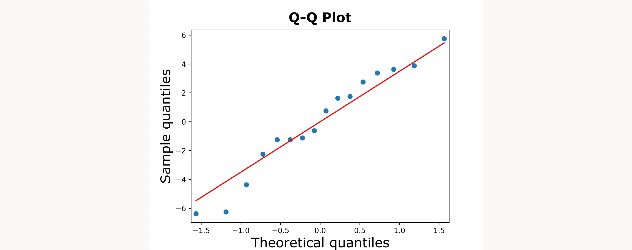
To test whether the residuals follow a normal distribution, we’ll use a Q-Q plot. This is important because ANOVA’s statistical tests (like p-values) assume normality. If the residuals aren’t normal, the p-values might be unreliable.

# Q-Q plot of residuals
sm.qqplot(residuals, line="s")
plt.title("Q-Q Plot of ANOVA Residuals")
plt.show()

Code explanation:

• sm.qqplot() creates a quantile-quantile plot comparing residuals to a theoretical normal distribution
• line="s" adds a reference line to help visualize normality
• If the points fall roughly along the line, the normality assumption is satisfied

The output will be the following figure:

Testing Independence

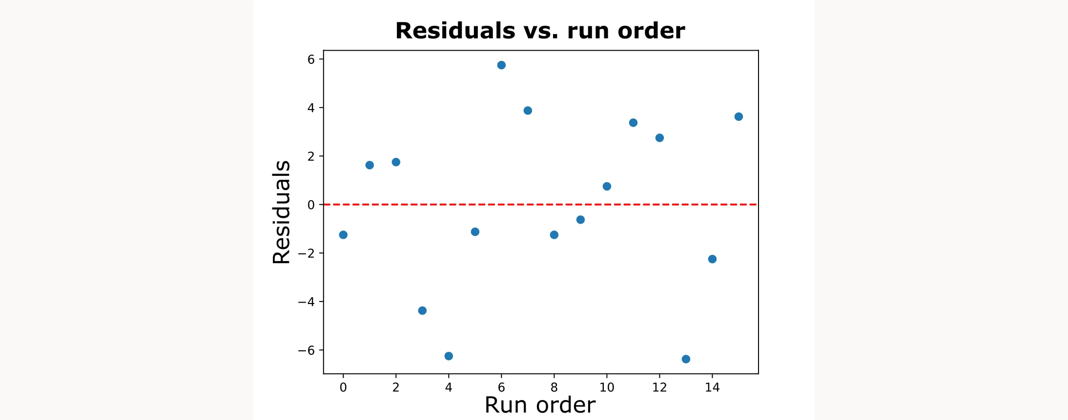
Next, we’ll test for independence by plotting residuals against the run order.

# Residuals vs run/order (look for patterns/trends)
plt.scatter(df.index, residuals)
plt.xlabel('Run Order')
plt.ylabel('Residuals')
plt.title('Residuals vs Run Order')
plt.axhline(0, color='red', linestyle='--')
plt.savefig("Residuals_vs_RunOrder.svg")
plt.show()

Code explanation:

• plt.plot(df["order"], residuals, marker="o", linestyle="-") creates a line plot of residuals against run order
• plt.axhline(0, color='red', linestyle='--') adds a red, horizontal dashed line at zero as a reference
• We’re looking for random scatter around zero. Any trends or patterns suggest the independence assumption is violated

This is how the output figure will look like:

Testing Equal Variance

# Residuals vs fitted values (look for “funnel” shapes)
plt.scatter(fitted, residuals)
plt.axhline(0, color='red', linestyle="--")
plt.title("Residuals vs Fitted")
plt.xlabel("Fitted values")
plt.ylabel("Residuals")
plt.savefig("Residuals_vs_Fitted.svg")
plt.show()

Code explanation:

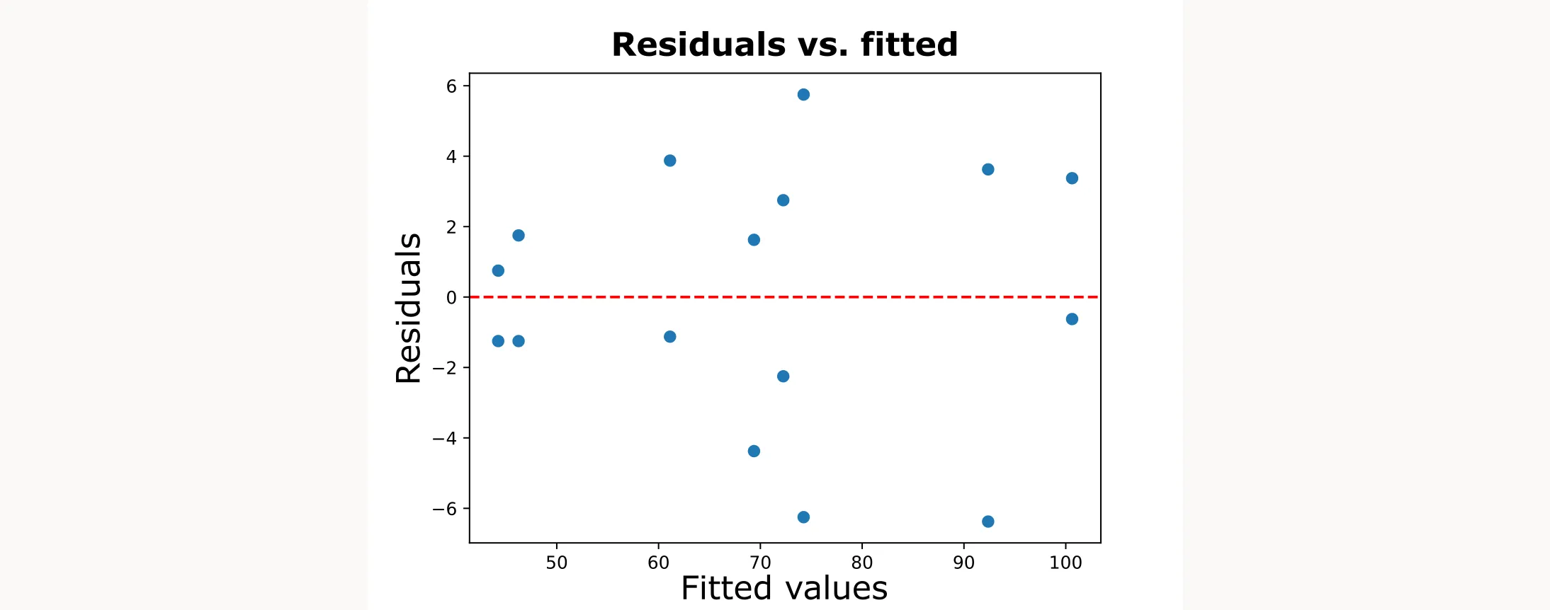
• plt.scatter(fitted, residuals) creates a scatter plot of residuals against fitted values
• plt.axhline(0, color='red', linestyle="--") adds a red, horizontal dashed line at zero as a reference
• We’re looking for a constant spread of residuals around zero. A “funnel” shape (narrow at one end and wide at the other) indicates a violation of the equal variance assumption

This is how it looks like:

Adding Quadratic Terms for Advanced Designs

If you’re working with a central composite design (CCD) or other response surface methodology, you can add quadratic terms to capture non-linear relationships. The anlysis as well as the testing of ANOVA assumptions will be the same:

# Adding quadratic terms
# Note: I(T**2) syntax tells Python to treat T**2 as a mathematical operation
formula_quad = 'Filtration_rate ~ T + CoF + RPM + T:CoF + T:RPM + I(T**2) + I(CoF**2) + I(RPM**2)'

model_quad = ols(formula_quad, data=df).fit()

anova_results_quad = sm.stats.anova_lm(model_quad, typ=2)  # Type II ANOVA
print(anova_results_quad)

Important note: You can only meaningfully add quadratic terms if your experimental design includes center points or multiple levels for each factor. A simple two-level factorial design doesn’t provide enough information to estimate quadratic effects reliably.

The I() function: This tells the formula parser to treat the expression inside as a mathematical operation rather than a formula operator. Without it, T**2 might be misinterpreted.

Up next:

<< Create a Fractional Factorial Design in Python >>

<< Create a Full Factorial Design in Python >>