Developing new materials often involves testing multiple candidates to find the best performer. For example, you might compare 19 different diluents to see how they each affect a resin’s viscosity. But testing every combination at 4 concentrations means 76 experiments.

Do we really need all 76 measurements? Or can we predict the performance of all 19 candidates from a smaller, well-chosen subset?

We’ll compare three strategies for mapping this landscape: a random baseline, a physics-inspired “expert approach”, and an adaptive Active Learning strategy. All three aim to cut the time spent in the lab significantly.

The setup

We already have all 76 viscosity values in our dataset, so we can run this as a simulation. Instead of going to the lab, we “measure” any experiment by looking up its result.

For each strategy, we track how well the model predicts the unmeasured points using R² and RMSE. The goal is high R² with as few measurements as possible.

What we’re working with

The dataset consists of 19 diluents, each measured at 4 concentrations (10, 15, 20, 30 g per 100 g resin). The table below lists all diluents and the four physical features used for the predictions:

Diluent	EEW (g/eq)	Functionality	Viscosity 23 °C (mPa·s)	Density (g/cm³)
Diluent A	182	0	29.2	0.935
Diluent B	220	1	4.0	0.890
Diluent C	285	1	7.5	0.900
Diluent D	150	2	20.0	1.060
Diluent E	135	2	15.0	1.110
Diluent F	198	0	18.2	0.935
Diluent G	245	0	18.2	0.935
Diluent H	296	0	68.3	0.975
Diluent I	90	2	20.0	1.050
Diluent J	310	0	50.0	0.975
Diluent K	400	0	50.0	0.970
Diluent L	290	0	15.0	0.920
Diluent M	330	0	14.0	0.920
Diluent N	250	0	20.0	0.920
Diluent O	330	0	14.0	0.920
Diluent P	500	1	50.0	0.970
Diluent Q	0	0	55.0	0.930
Diluent R	0	0	29.4	0.975
Diluent S	200	0	38.8	0.940

To get a feel for the data, here are three representative viscosity-concentration curves. Each diluent follows a roughly exponential decay: viscosity drops steeply at low concentrations and then flattens out.

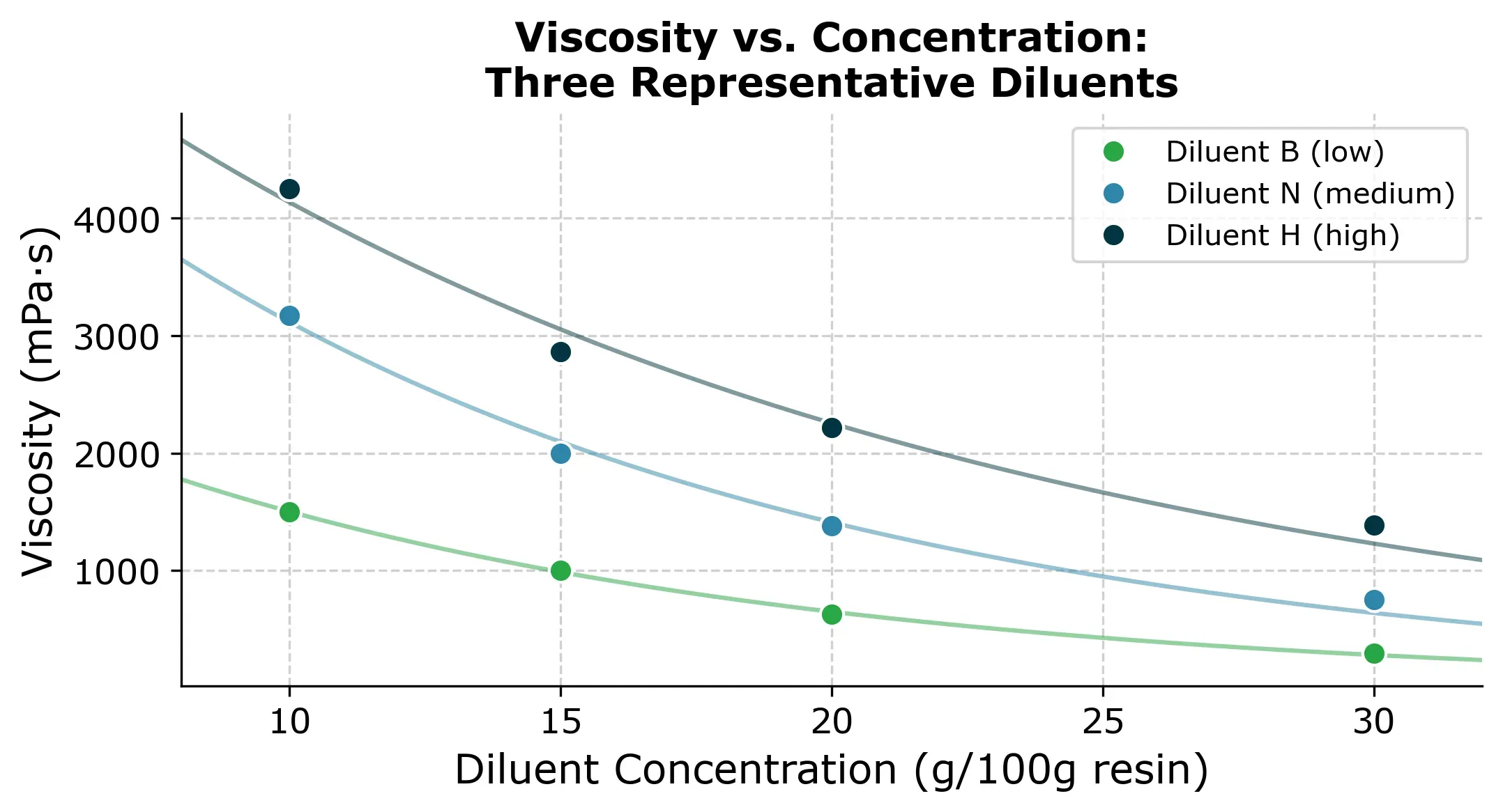
These curves are what we’re trying to reconstruct. Each diluent has a different starting viscosity and a different decay rate. If we had to measure all 76 points, that’s roughly a full day of lab work. So the question is can we get away with less?

That means we need to create a model that can predict the viscosity of all 19 diluents from a smaller, well-chosen subset of measurements.

Establishing the baselines

The random baseline

The simplest strategy is to pick experiments at random, one at a time, measure the viscosity, train a model (in this case a Gaussian Process model) and track how the prediction quality improves.

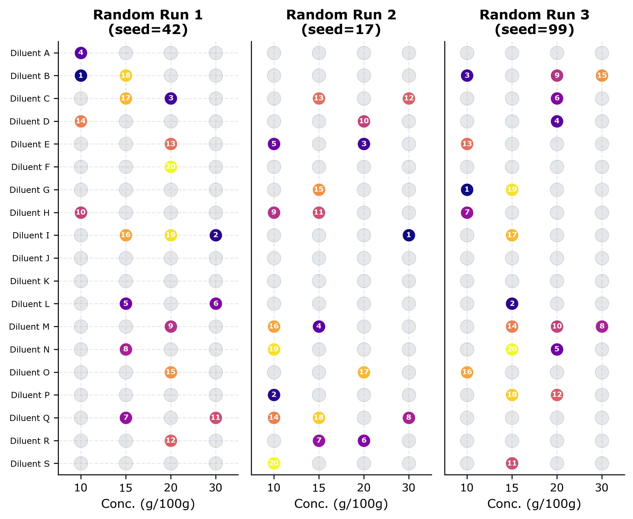
Since the order in which we pick random experiments matters, we repeat the process 10 times with different random orderings and average the results. This gives us a stable estimate of how random selection performs on average. Any single random run can look much better or much worse.

Three examples of random selection grids are shown below. Each grid shows which experiments were “measured” (numbered by order) and which remain unmeasured (gray). Notice how the random selection is already covering the design space quite nicely, but some runs cluster in certain rows and some diluents are not measured at all (for no obvious reason).

The learning curve below shows how R² and RMSE evolve as more random measurements are added.

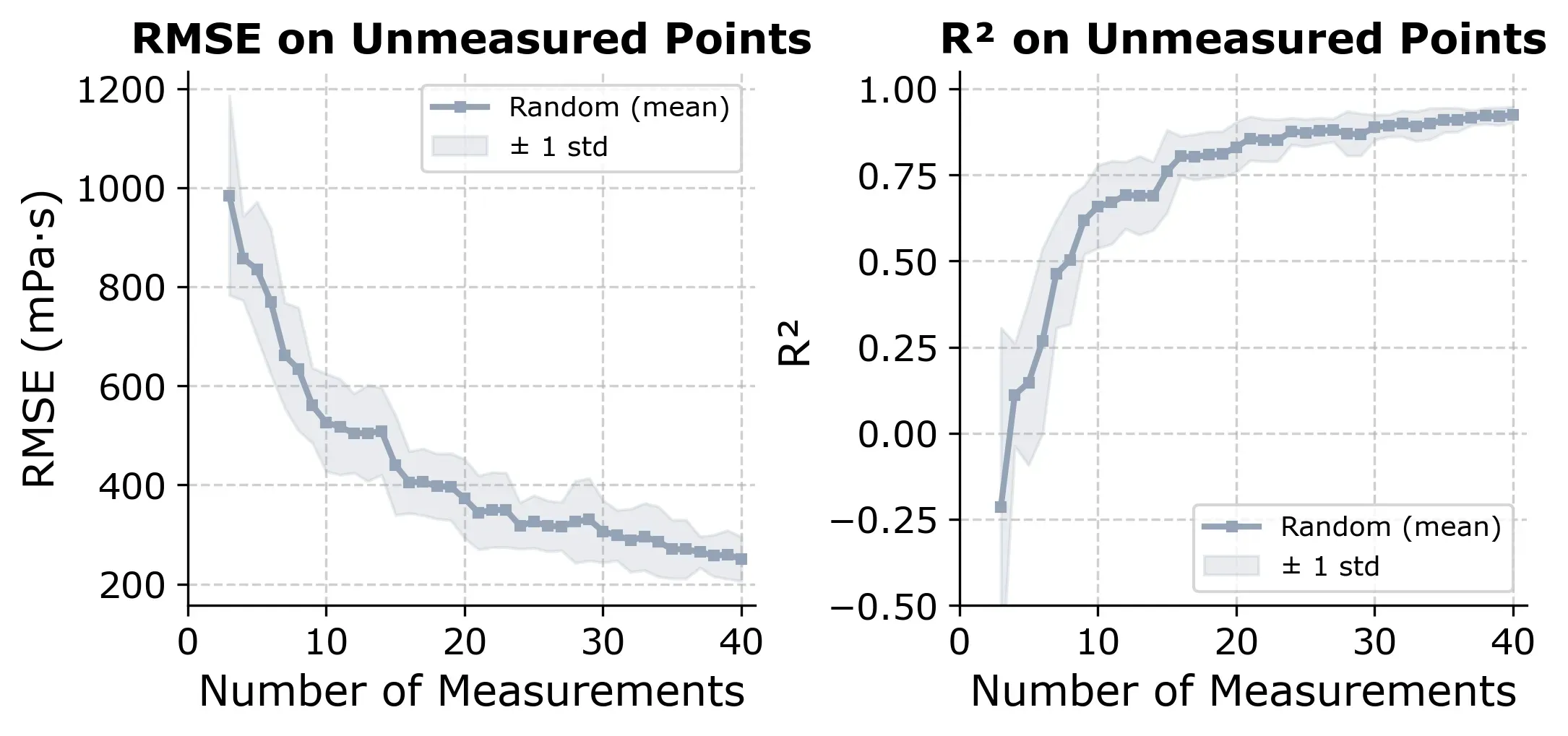
If we select points randomly, we reach R² ≈ 0.80 at around 20 to 25 measurements, which is about 30% of the design space. It’s a useful baseline. Any smarter strategy should beat this consistently.

The expert approach

Before reaching for machine learning, let’s think about what a formulator with domain knowledge could do.

Following considerations:

1. Viscosity follows an exponential decay with diluent concentration: $\eta = A \cdot \exp(-B \cdot c)$. This Arrhenius-like relationship is a standard model in polymer science.
2. A single measurement for each diluent captures the individual diluent behavior.

That means we can:

1. Pick one diluent and measure all 4 concentrations (4 measurements)
2. Fit the exponential model $\eta = A \cdot \exp(-B \cdot c)$ to these 4 points, which gives us the decay rate $B$
3. Measure the anchor point (viscosity at 10 g/100g) for all other 18 diluents (18 measurements)
4. Calculate each diluent’s pre-factor: $A_i = \eta_i(10) / \exp(-B \cdot 10)$
5. Predict all remaining concentrations: $\eta_i(c) = A_i \cdot \exp(-B \cdot c)$

Total cost: 22 measurements (4 + 18). That’s 29% of the full design space, and it gives us predictions for the remaining 54 points.

Note: In a real lab, you’d want to add a few verification measurements on top, picking a handful of diluent-concentration combinations at random and checking whether the predictions hold. So the true cost is closer to 25 to 30 measurements. But the core strategy needs only 22.

How well does it work?

Since the result depends on which diluent we start with, we simulate all 19 possibilities and report the distribution.

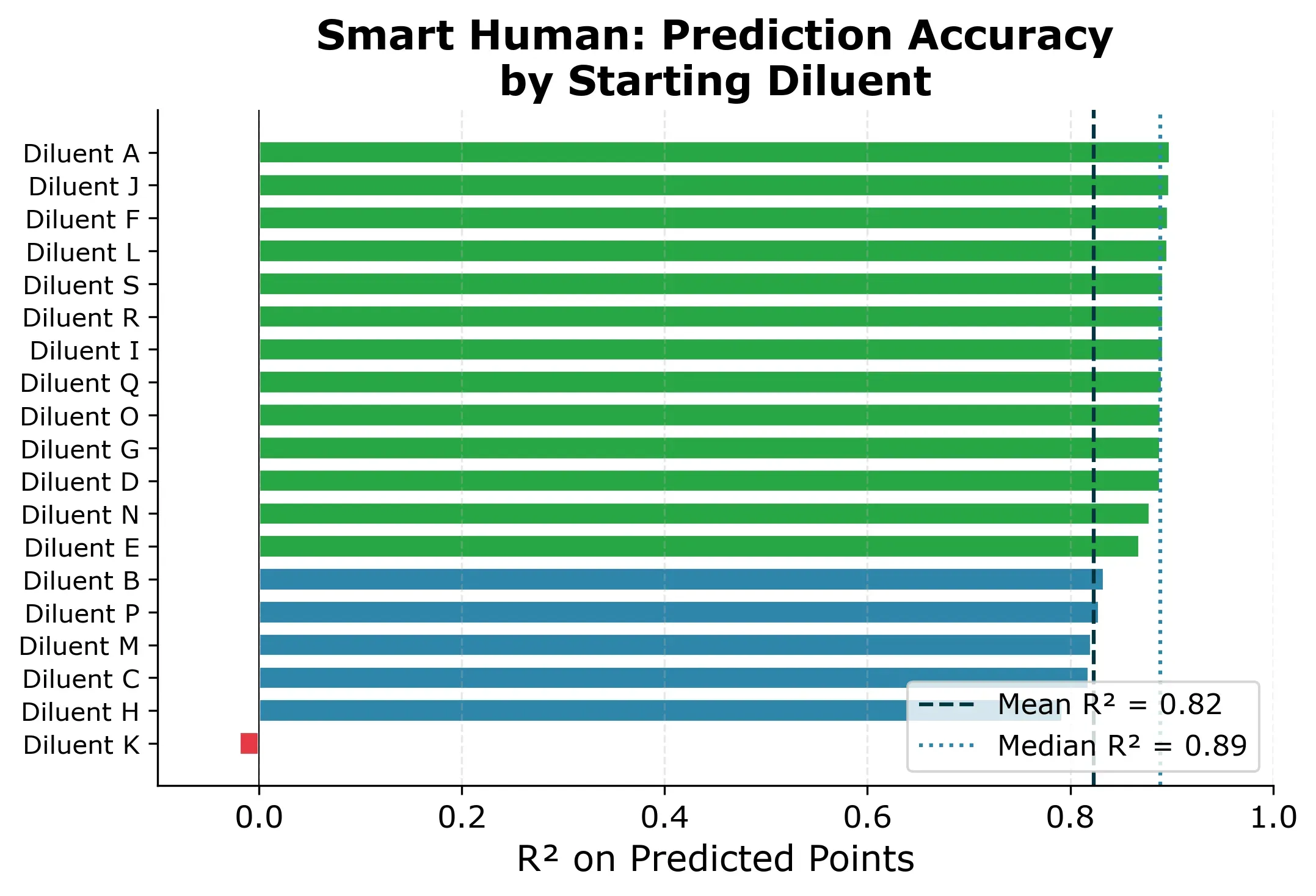
The result: R² = 0.89 median across starting diluents, with RMSE around 200 mPa·s. Most starting diluents give very consistent results. 15 out of 19 produce R² between 0.83 and 0.90.

One diluent is different though. If we picked Diluent K as the starting diluent, we would get a near-useless model (R² ≈ 0) and all predictions would be slightly off as you can see in Figure 5 below.

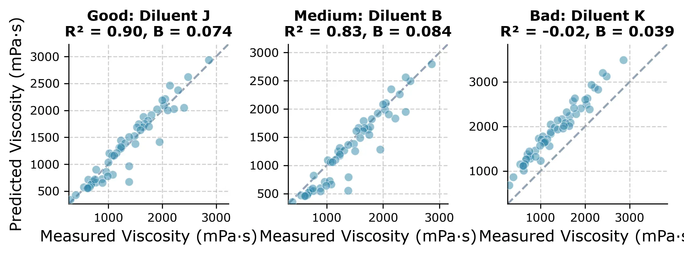
The reason is that with Diluent K you get an unusually flat viscosity-concentration curve ($B \approx 0.04$, compared to the typical $0.07$) as you can in the next plot.

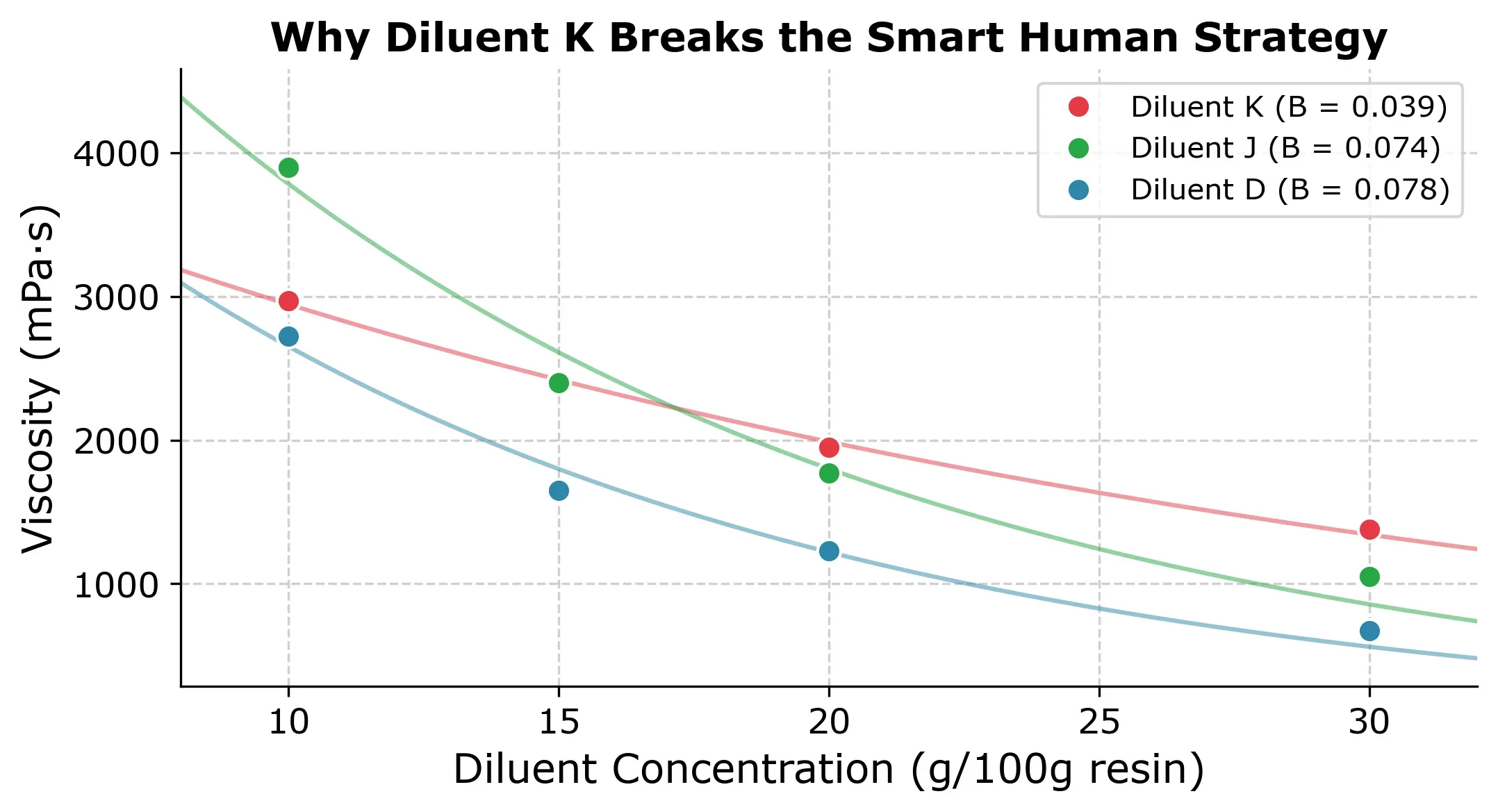
This is the core weakness of the approach. It assumes all diluents share a similar exponential decay. When that assumption holds, the results are excellent but when it doesnt you might lose trust in the modeling approach and fall back to the conventional approach of measuring all concentrations for each diluent.

Active learning with BayBE

BayBE is a Python package for experimental optimization. It’s normally used to find the best experiment, but it can also be used for something called active learning. Instead of searching for the optimum, we want it to find the most informative measurements that would reduce the models total prediction uncertainty the most. To do that, we need to pick the correct acquisition function. In this case we pick qNIPV (Noiseless Information-based Potential of Value).

The workflow is like this:

• After each measurement, the Gaussian Process has predictions and uncertainty estimates for every unmeasured point
• qNIPV evaluates: “if I measured point X, how much would my total uncertainty across all unmeasured points decrease?”
• It picks the point with the highest expected uncertainty reduction
• Early on, this means diverse points spread across different diluents and concentrations
• Later, it fills in gaps where the model is least confident

What sets this apart from both the random baseline and the smart human approach is that each choice depends on everything measured so far. It’s adaptive, and it requires no domain knowledge about viscosity, exponential decays, or anchor points. In addition to that, it is more robust than the expert approach as we saw with Diluent K.

How it performs

BayBE uses a two-phase strategy: the first 3 experiments are selected by Farthest Point Sampling (FPS) to spread across the feature space, then qNIPV takes over for the remaining experiments. The plot below shows how fast the model improves compared to the two other approaches.

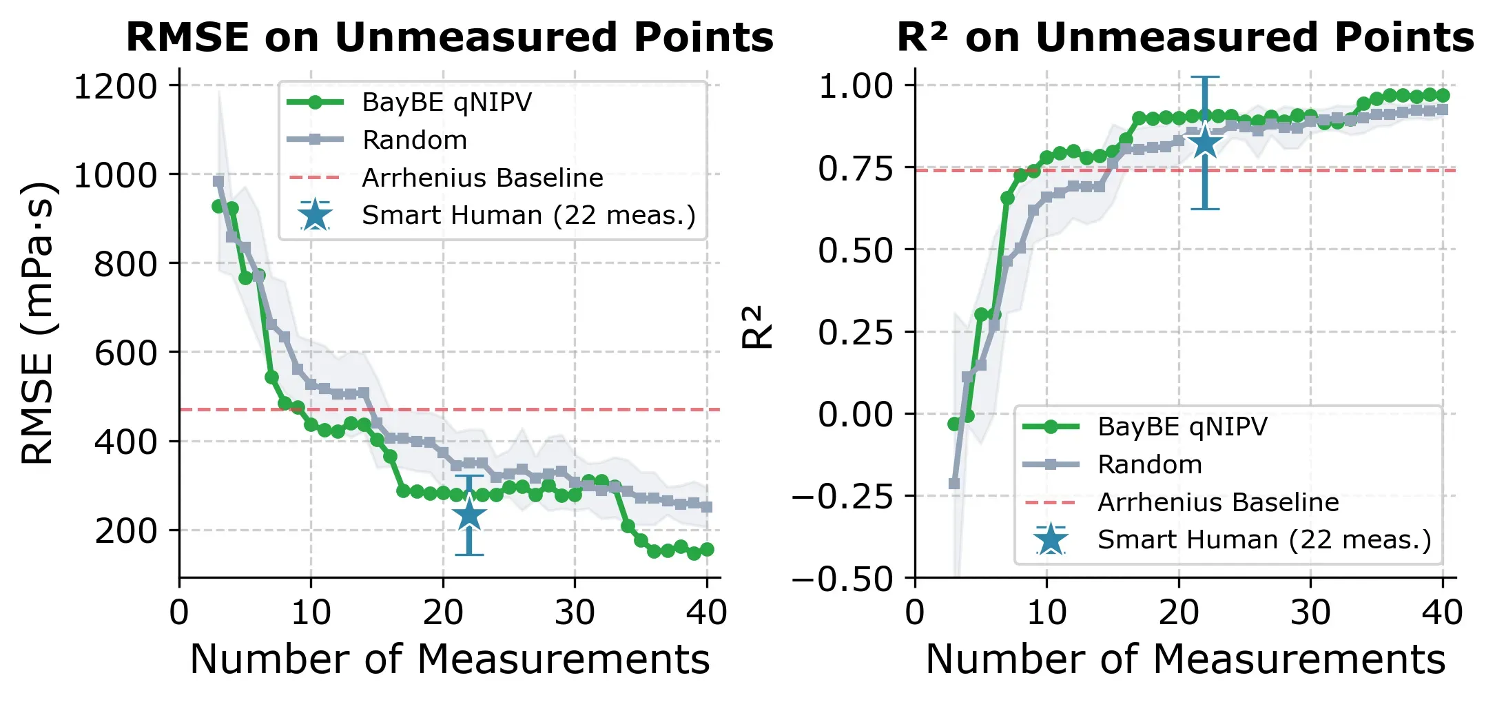
BayBE (green) reaches R² ≥ 0.80 faster than random selection and with less variance. The expert approach (blue star at 22 measurements) achieves a strong median R² of 0.89, but its wide error bar reflects the risk of picking an outlier like Diluent K.

Here are the key thresholds for the active learning approach:

Target	BayBE (experiments needed)	% of data
R² ≥ 0.80	16	21%
R² ≥ 0.85	17	22%
R² ≥ 0.90	19	25%

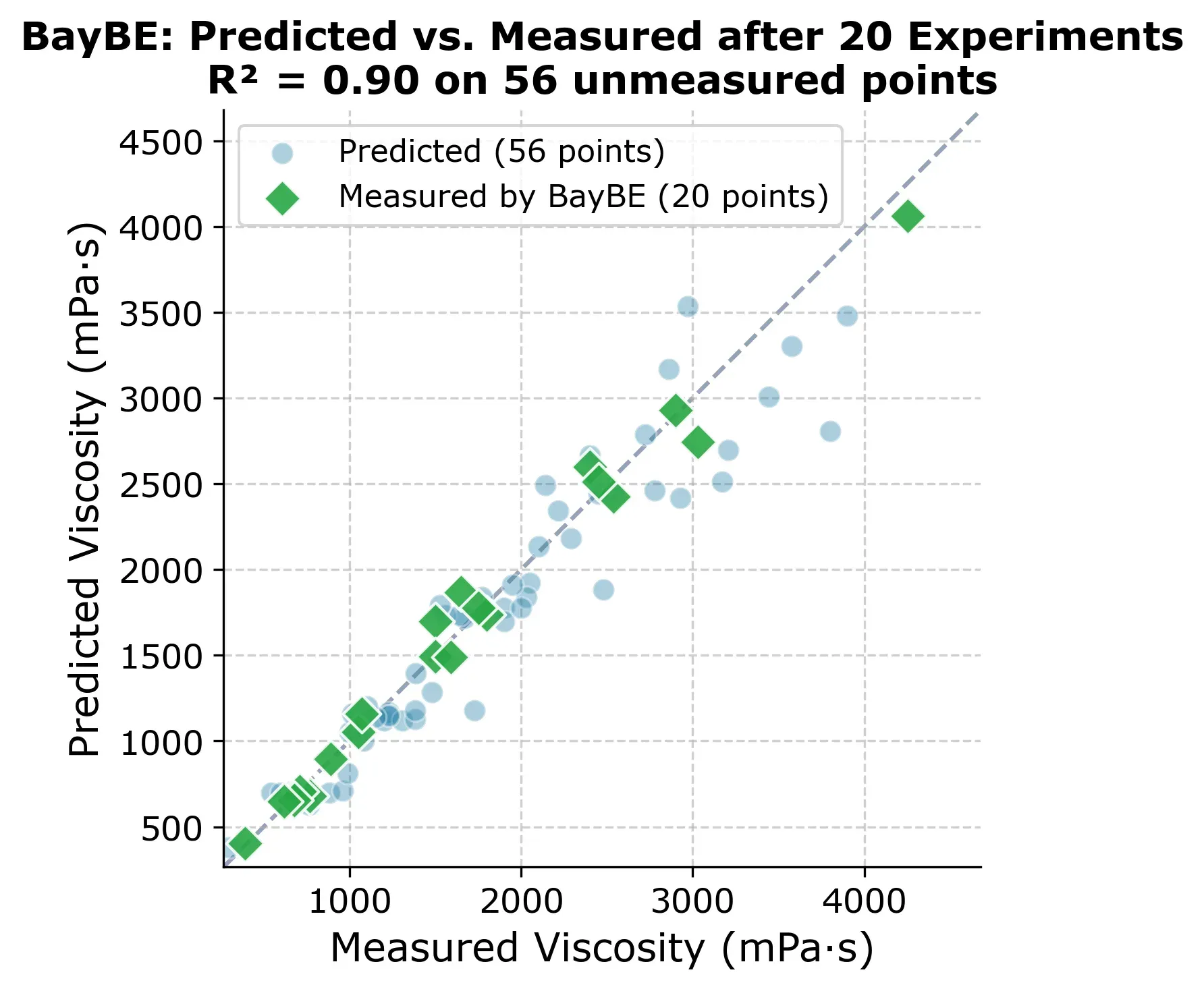
At 20 experiments, BayBE already has a solid model of the entire design space. The figure below shows predicted vs. measured for all 76 points, with the 20 experiments BayBE chose highlighted as green diamonds.

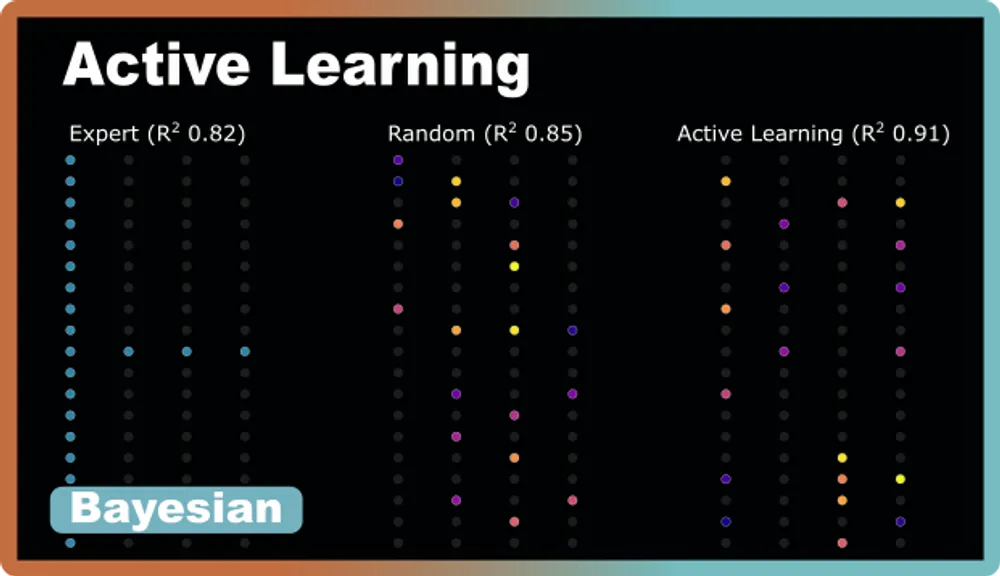
But which experiments did BayBE actually choose? The selection grid below shows the order in which points were picked.

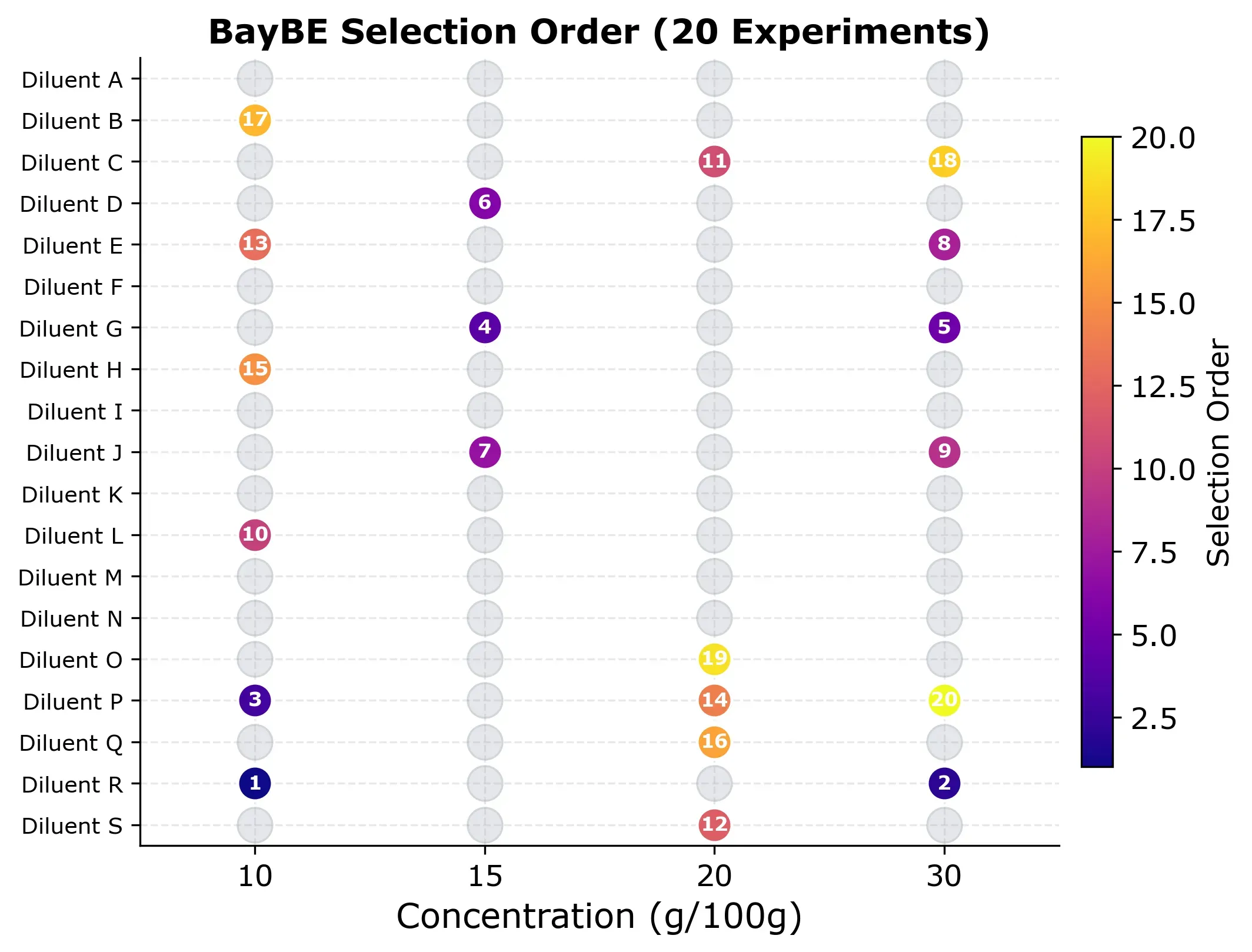
The pattern is worth looking at. Early experiments (dark colors) spread across different diluents and concentrations as BayBE explores broadly. Later experiments (bright colors) fill in specific gaps where the model is least confident. No concentration is over-represented, and the algorithm naturally avoids clustering.

Takeaway

All three approaches give accurate enough predictions so that testing every diluent at every concentration is simply more work than it needs to be.

Random selection and the expert approach are the simpler options. The expert approach is especially intuitive. It requires domain knowledge but can be done with a spreadsheet. However, both come with an element of luck. For random selection, it is which points happen to get picked, and for the expert approach it is which starting diluent you choose.

The active learning approach is more reliable and performs slightly better. It removes the luck factor, and you can apply it to all kinds of problems without needing to build a physical model first. The trade-off is that it requires some software setup and basic Python skills.

Whichever approach you go with, the key is to be deliberate about which experiments you run instead of defaulting to measuring everything.

Up next

<< Understanding Bayesian Optimization >>

<< Getting Started with Bayesian Optimization (BayBE) >>