I’ve covered what Bayesian Optimization is, how it performs on real lab data, and the technical details of surrogate models and acquisition functions in previous posts. We discussed how Bayesian Optimization uses a probabilistic model (the surrogate) to predict where good experiments might be, and an acquisition function to decide which experiment to run next. The surrogate learns from your data and provides uncertainty estimates, while the acquisition function balances exploring uncertain regions with exploiting promising areas. Now we’ll implement this in Python.

I want to show you how to actually get started with Bayesian Optimization. For this, I’ll use BayBE, a Python package for experimental optimization specifically designed for materials science problems. The BayBE documentation is quite extensive and I recommend reading it for more details. However, in this blog post I’ll cover the absolute basics to get you started and provide you a template that you can use.

I also created an AI assistant that can help you get started with BayBE. You can use it to generate the code for your specific problem. Here are two example prompts:

Simple example (like this tutorial): I want to optimize yield using BayBE. I have 2 continuous parameters (xi1 from 0 to 10, and xi2 from 0 to 1000). My target is to maximize yield. Use a Gaussian Process surrogate with qLogEI acquisition function, and start with 3 random initial experiments.

Complex example: I want to optimize reaction conversion using BayBE. I have 3 continuous parameters (temperature 20-80°C, pressure 1-5 bar, time 10-120 min), 2 categorical parameters (catalyst type: A/B/C, solvent: water/ethanol/acetone), and 1 discrete parameter (stirring speed: 100/200/300/400 rpm). My target is to maximize conversion. Use random sampling for 5 initial experiments.

How BayBE structures the workflow

BayBE organizes everything around a Campaign object. A campaign contains your search space definition, your objective, and the strategy for selecting experiments. You feed it measurement data, and it recommends the next experiments to run.

The workflow looks like this:

1. Define what you’re searching over (parameters and their ranges)
2. Specify what you’re trying to optimize (the target)
3. Choose a recommendation strategy (the algorithm)
4. Create the campaign object (this bundles everything together in Step 5)
5. Run the optimization loop: get recommendations, run experiments, add measurements, repeat

Let’s walk through a concrete example.

Step 1: Define the objective function

For this tutorial, we’ll use a test function that simulates a yield optimization problem. In practice, this would be your actual experimental measurements.

import numpy as np
import pandas as pd
import matplotlib.pyplot as plt
from baybe import Campaign
from baybe.parameters import NumericalContinuousParameter
from baybe.searchspace import SearchSpace
from baybe.targets import NumericalTarget
from baybe.recommenders import BotorchRecommender, TwoPhaseMetaRecommender, RandomRecommender
from baybe.surrogates import GaussianProcessSurrogate
from baybe.acquisition import qLogEI

def yield_fn(xi1, xi2):
    xi1, xi2 = float(xi1), float(xi2)
    x1_t, x2_t = 3 * xi1 - 15, xi2 / 50.0 - 13
    c, s = np.cos(0.5), np.sin(0.5)
    x1_r = c * x1_t - s * x2_t
    x2_r = s * x1_t + c * x2_t
    y = np.exp(-x1_r**2 / 80.0 - 0.5 * (x2_r + 0.03 * x1_r**2 - 40 * 0.03)**2)
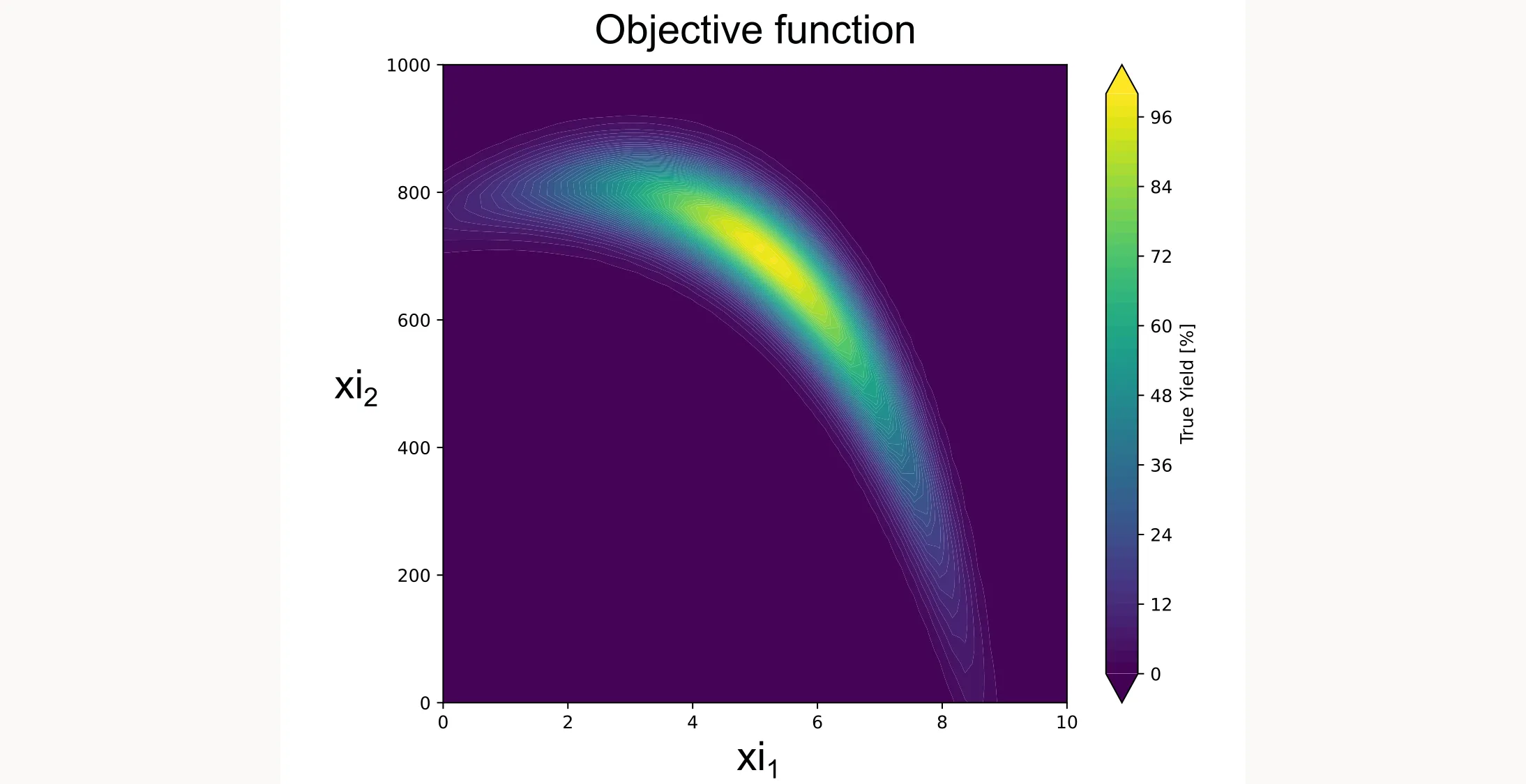
    return 100.0 * y

This function creates a smooth landscape with a global optimum, similar to what you might see with temperature and concentration effects in a real chemical system. Don’t worry about the specifics or the math behind it. We just want to create a realistic-looking test function. I plotted it for you as a contour plot below.

Step 2: Define the search space

You specify what parameters you can control and their valid ranges:

parameters = [
    NumericalContinuousParameter(name="xi1", bounds=(0, 10)),
    NumericalContinuousParameter(name="xi2", bounds=(0, 1000)),
]
searchspace = SearchSpace.from_product(parameters=parameters)

For this tutorial, xi1 and xi2 are generic parameters, not tied to specific physical quantities. In your real application, these might be temperature, concentration, reaction time, or any other variables you can control.

BayBE supports several parameter types (continuous, discrete, categorical), but in this case we just use continuous parameters.

Step 3: Configure the surrogate and acquisition function

Here’s where you choose how the algorithm models your system and makes decisions:

surrogate_model = GaussianProcessSurrogate()
acquisition_function = qLogEI()

Gaussian Process is the standard surrogate for many applications. BayBE also supports other surrogates like Random Forest (RandomForestSurrogate) or NGBoost (NGBoostSurrogate) and even more specialized surrogates.

qLogEI (Log Expected Improvement) is an acquisition function that balances finding better points (exploitation) with exploring uncertain regions (exploration). Expected Improvement calculates how much better a point is expected to be compared to your current best result. It automatically balances exploration (trying uncertain regions) and exploitation (trying near your current best) by weighing potential improvement against uncertainty. The ‘Log’ version uses a logarithmic transformation that can be more numerically stable and robust, especially in batch settings. The ‘q’ prefix means ‘quasi-Monte Carlo batch’, which allows it to suggest multiple experiments simultaneously by considering how informative each combination would be together. This is useful if you can run experiments in parallel (e.g., multiple reaction vessels). Set batch_size=N when calling recommend() to get N suggestions at once.

It is a good default for most applications. But again, there is a whole list of acquisition functions available.

Step 4: Define the recommender strategy

One of BayBE’s smart features is the two-phase approach:

recommender = TwoPhaseMetaRecommender(
    initial_recommender=RandomRecommender(),
    recommender=BotorchRecommender(
        surrogate_model=surrogate_model,
        acquisition_function=acquisition_function
    ),
    switch_after=3
)

Why the two phases? Bayesian optimization needs initial data to build its model. Starting with a few random experiments (here, 3) gives the algorithm something to learn from before it starts making strategic recommendations.

The RandomRecommender is mainly for continuous search spaces. For discrete search spaces, there are more sophisticated options. You can also use data from, for example, a fractional factorial design you already ran previously.

After those initial experiments, it switches to the BotorchRecommender that uses your specified surrogate and acquisition function.

Step 5: Create the campaign

Now you bundle everything together into a Campaign object:

target = NumericalTarget(name="yield")
campaign = Campaign(
    searchspace=searchspace,
    objective=target,
    recommender=recommender
)

It is your central control point. It tracks all measurements, manages the model, and handles recommendations.

Step 6: Run the optimization loop

Now the optimization begins:

print("Starting BayBE Optimization...")
for i in range(15):
    rec = campaign.recommend(batch_size=1)
    xi1, xi2 = rec["xi1"].iloc[0], rec["xi2"].iloc[0]
    y = yield_fn(xi1, xi2)
    rec["yield"] = y
    campaign.add_measurements(rec)
    print(f"Trial {i+1:02d}: xi1={xi1:6.2f}, xi2={xi2:7.2f} | Yield = {y:6.2f}%")

The for loop here is only for this tutorial where we use the artificial yield function. In a real application, you wouldn’t need a for loop. You would run the experiments in the lab or plant and add the results to the campaign manually. You’d be the for loop yourself, running one iteration at a time as your experiments complete.

Each iteration:

1. recommend() suggests the next experiment
2. You run the experiment (here, evaluating yield_fn)
3. You add the result back to the campaign with add_measurements()
4. The algorithm updates its model and becomes smarter

Step 7: Extract and visualize results

We use a cumulative best plot to show how quickly we approach the optimum.

best_idx = campaign.measurements["yield"].idxmax()
print(f"\nBest Yield: {campaign.measurements.loc[best_idx, 'yield']:.4f}%")

yield_values = campaign.measurements["yield"].values
cum_max_values = np.maximum.accumulate(yield_values)

plt.figure(figsize=(10, 6))
plt.scatter(range(1, len(yield_values) + 1), yield_values,
            color='green', alpha=0.4, label='Individual Trials')
plt.plot(range(1, len(cum_max_values) + 1), cum_max_values,
         color='green', marker='s', linewidth=2, label='Cumulative Best')
plt.title("Optimization Progress", fontsize=14)
plt.xlabel("Trial Number", fontsize=12)
plt.ylabel("Yield [%]", fontsize=12)
plt.grid(True, linestyle='--', alpha=0.6)
plt.legend()
plt.show()

It shows two things: the light green dots are the individual yield values from each trial, and the dark green line with squares tracks the best yield found so far at each step. This cumulative best line can only stay flat or go up, never down, because it always shows the highest yield you’ve achieved up to that point. It tells you how quickly you’re approaching the optimum. In a well-tuned optimization, this curve should flatten as you find the best region. In our case the curve does not yet flatten, because we only have 15 trials. However, we are already close to 100 % yield, which kind of is the optimum.

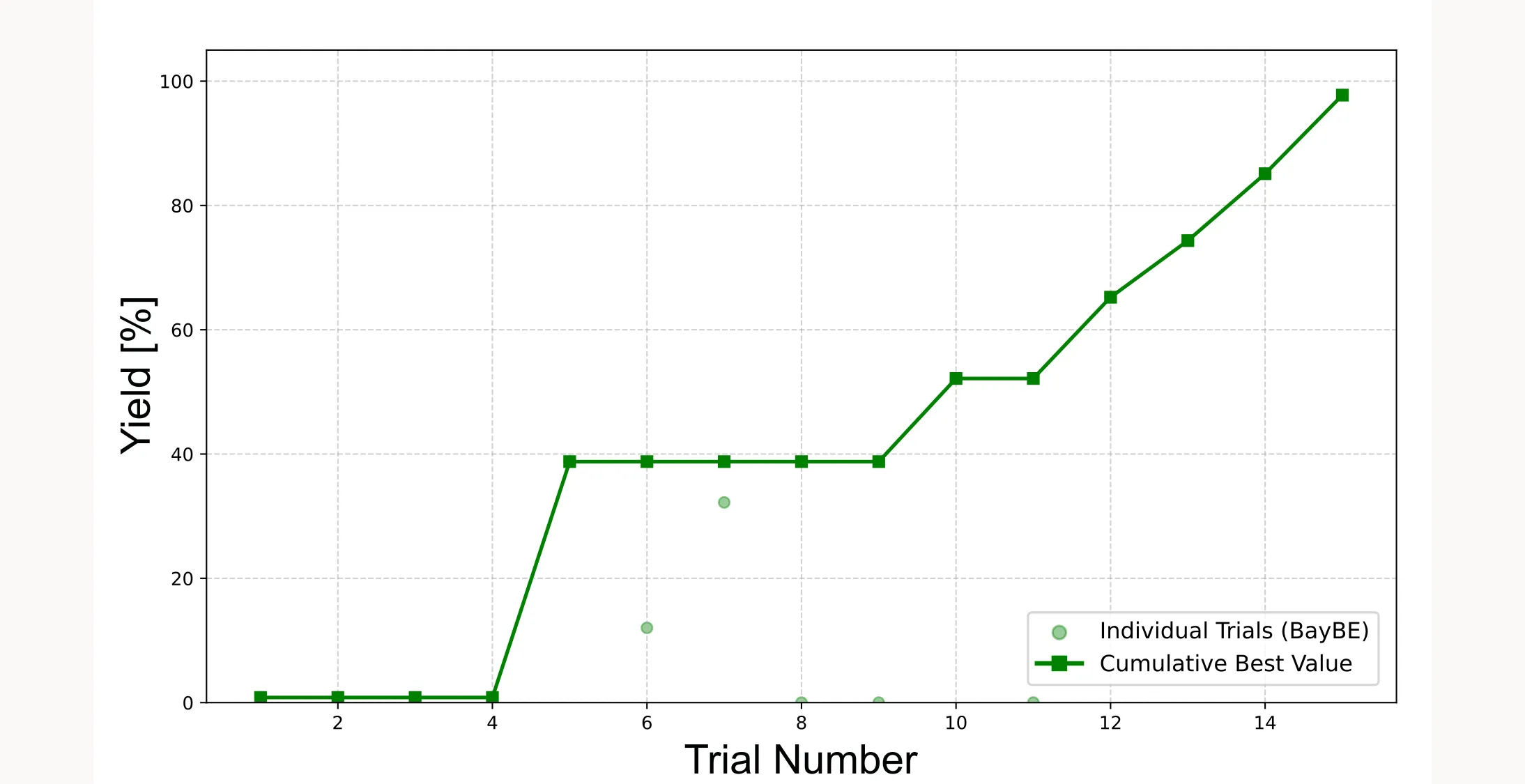
Important: Because the initial points are sampled randomly, the cumulative best plot will look different every time you run the optimization. Sometimes the algorithm will find the optimum faster, sometimes slower. Sometimes it will fail and not even come close to the optimum. It all depends on how lucky you are with the initial points.

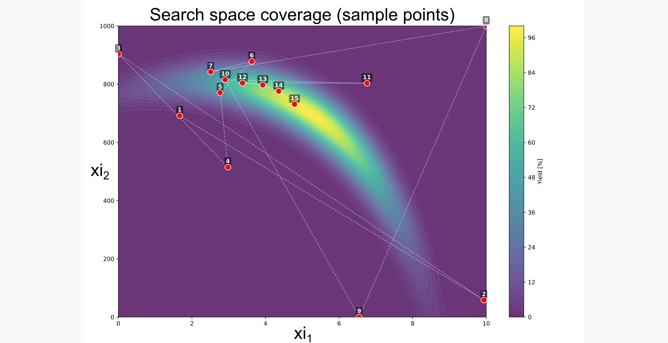
There are more ways to visualize the results, like shown below. You can see how the algorithm searches different locations initially but then quickly picks up on a path that will lead to the best yield.

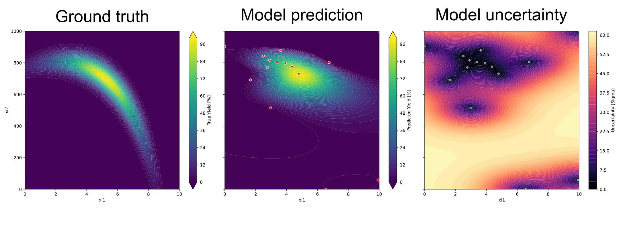
You can also visualize the surrogate model as well as the uncertainty of the model. But for this example, we’ll stop here.

If you want access to the full code, you can find it here.

Up next

<< A Technical Guide to Bayesian Optimization >>

<< Testing Bayesian Optimization for Lab Experiments >>