The Basics of Designing Better Experiments
How do you perform experiments?
Let’s stick with our previous filtration rate example and say we have two factors: temperature and pressure. You’d like to find their optimum settings to maximize the filtration rate in a chemical process. How exactly would you perform the experiments? How would you combine those two factors if, let’s say, we are testing temperature between 20 and 60 °C and pressure between 1 and 10 bar?
Below is an empty table you could fill in. I encourage you to actually do the exercise—it’s more interesting when you try it yourself.
| Run | Temperature (°C) | Pressure (bar) |
|---|---|---|
| 1 | ||
| 2 | ||
| … |
Here is an example of how you might set up the experiments:
| Run | Temperature (°C) | Pressure (bar) |
|---|---|---|
| 1 | 20 | 1 |
| 2 | 40 | 1 |
| 3 | 60 | 1 |
| 4 | 60 | 5 |
| 5 | 60 | 10 |
In this sequence, you first explore temperature at low pressure, then continue at higher pressures once you think 60 °C looks promising. This is a classic one-factor-at-a-time (OFAT) approach.
But here’s the catch: what if the combination of factors matters more than the factors alone? Maybe 40 °C only performs well at high pressure, or 60 °C is great at low pressure but not at high pressure. Those are the interactions we covered in our previous blog post that are so important. With OFAT, you completely miss them.
Visualizing the Design Space
Therefore, let’s try a different approach. Imagine a simple grid where temperature is on the x-axis and pressure on the y-axis. Each point on the grid represents a potential experiment.
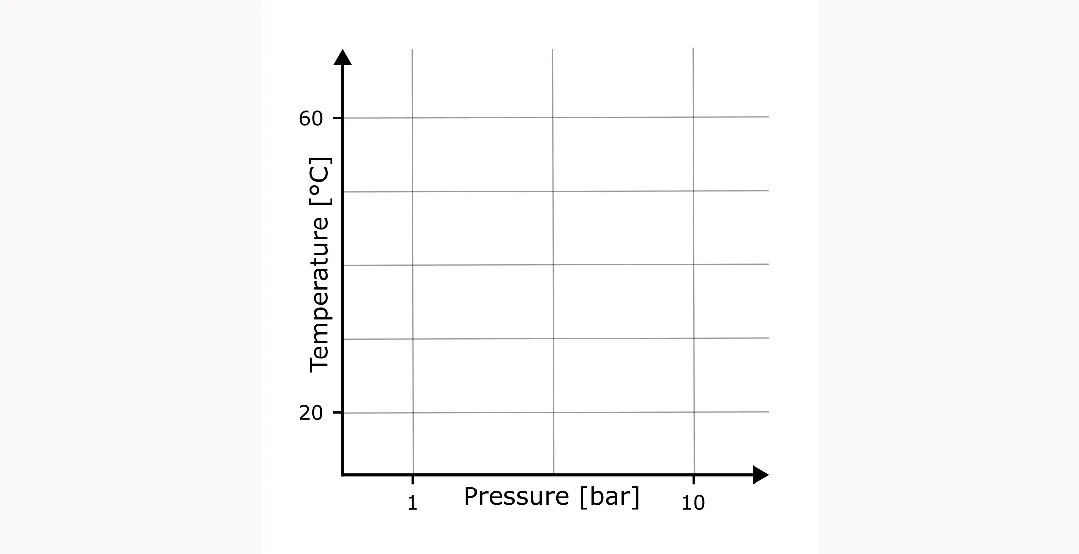
How would you arrange the experiments this time? Would you still take the OFAT approach? It looks like this:
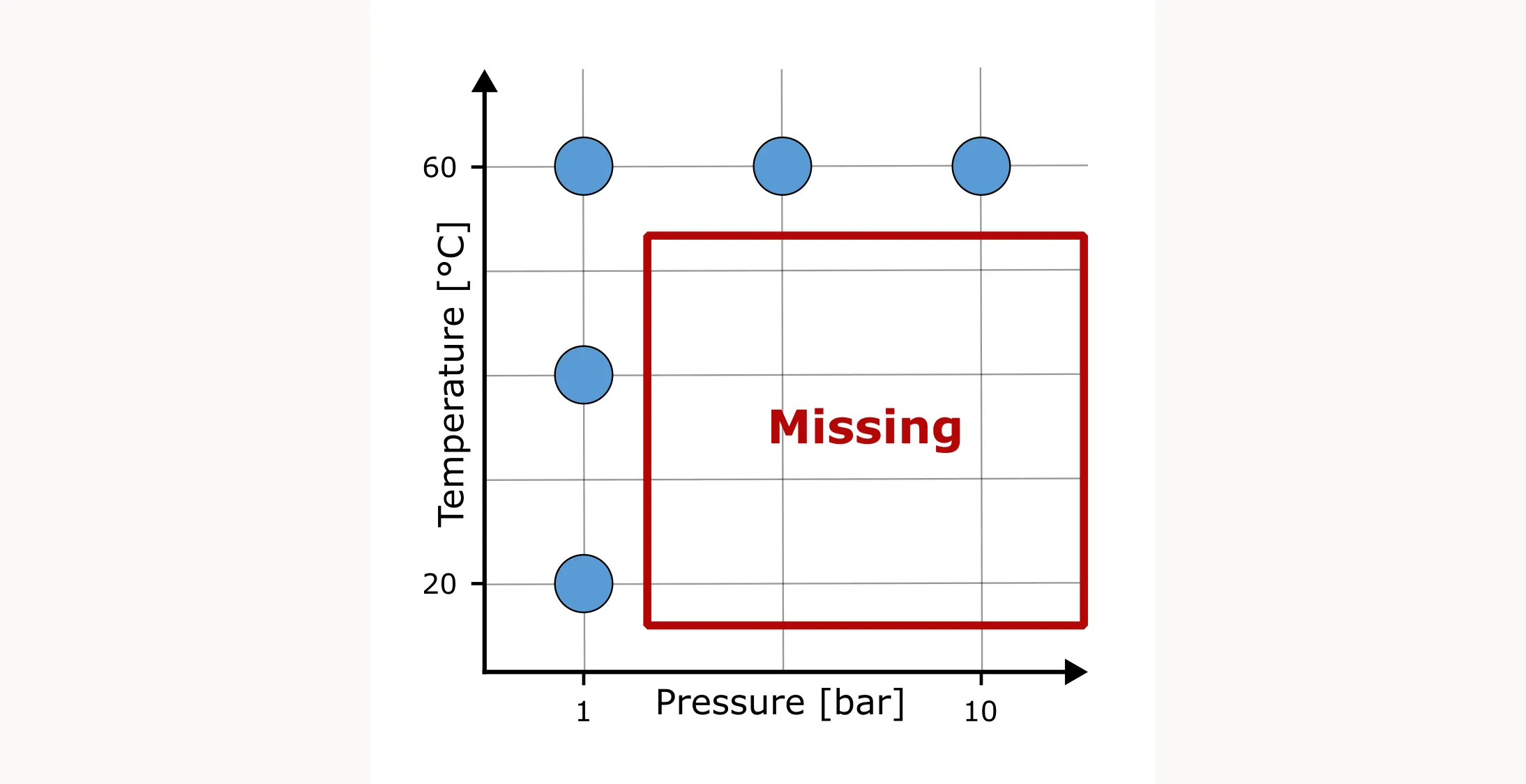
You’ll cover only a narrow slice of the design space and you would miss quite a lot of information.
A different approach would be to place your runs across the whole rectangle in a narrow grid. This way you get the most information possible and you cover the design space systematically. The problem though is that you need to perform a lot of experiments.
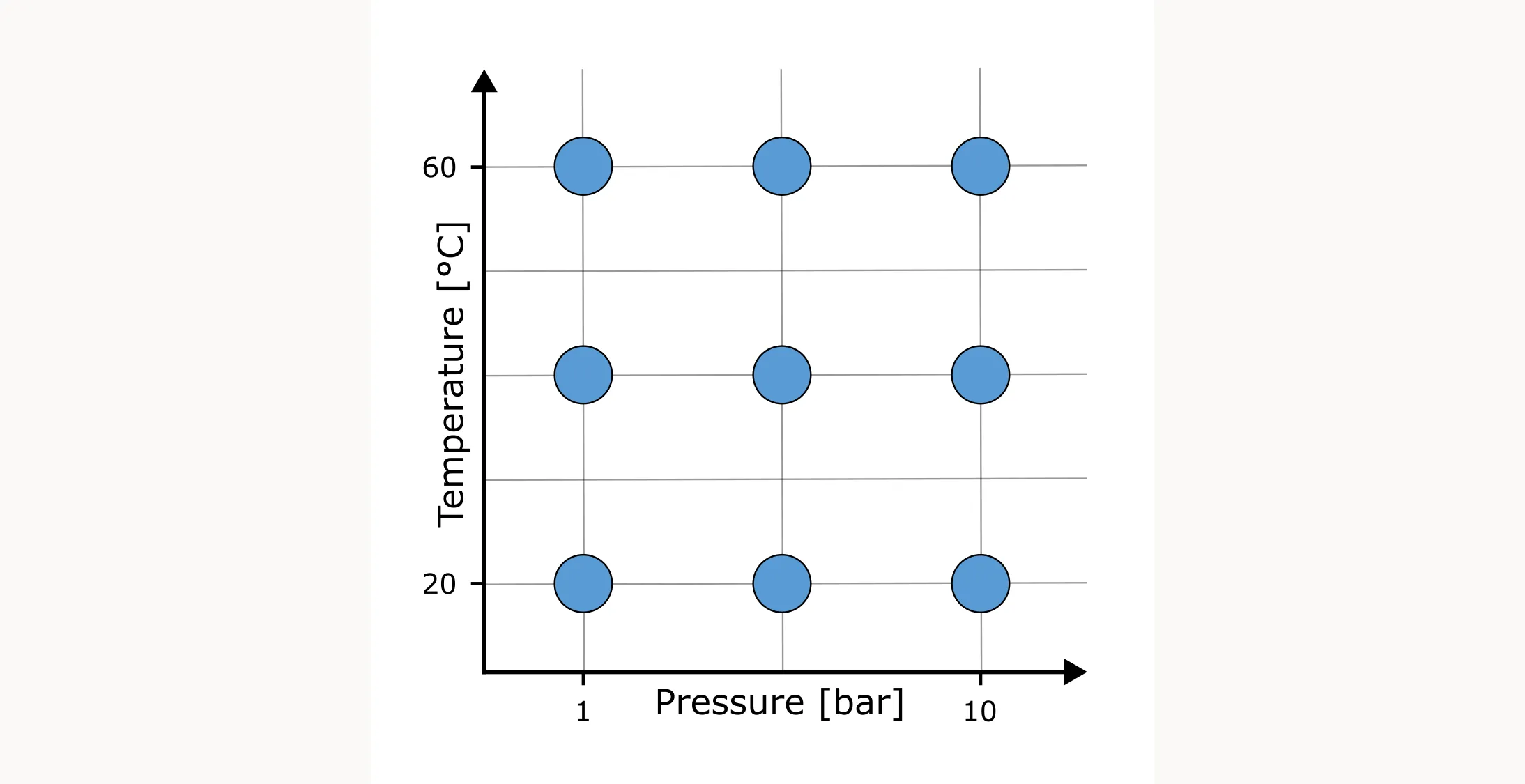
And this is the problem we are trying to solve with Design of Experiments (DoE). We want to cover the design space systematically, with as few experiments as possible, gaining as much information as possible. And one solution could look like this:
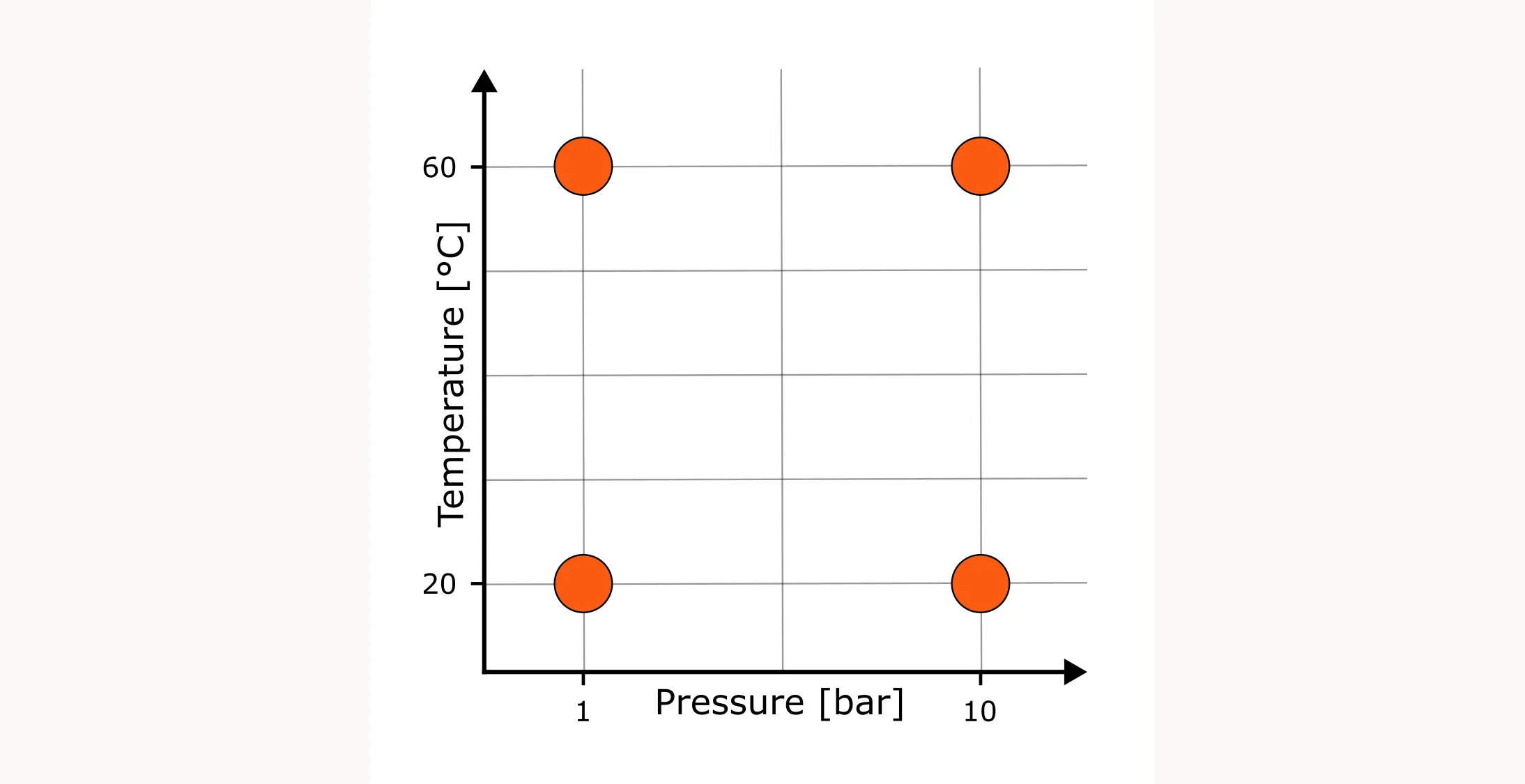
This design is called a full factorial design. Here, we test only the extremes and assume that the response changes approximately linearly between them. With two factors at two levels each, that means four experimental runs—covering all combinations of low and high temperature with low and high pressure. From these runs, we can estimate both the main effects and their interaction. This makes the full factorial design the simplest entry point into DoE.
Let’s take a detailed look at how a full factorial design works in the next blog post.