Foldover Designs
You’ve run a fractional factorial design, analyzed the results, and one of your factors shows a surprisingly large effect. But you know it’s confounded with a two-way interaction. You can’t tell from the data whether the main effect is real or whether the two-way interaction is inflating it.
A foldover design can help. Rather than running every missing experiment to complete the full factorial design, you run a carefully selected second batch of experiments to strategically untangle the confounded effects.
Ambiguous results with a resolution III design
Let’s set up a concrete example. Suppose you’re developing a coating and want to screen five process factors for their effect on pendulum damping (a measure of coating hardness):
- A — Curing Conditions
- B — Catalyst Type
- C — Catalyst Concentration
- D — Hardener Type
- E — Crosslinking Degree
You’re in the early screening phase. A full factorial design with five factors would require 2⁵ = 32 runs, which is too many. So you decide to run a 2⁵⁻² fractional factorial design with only 8 runs. This is a Resolution III design.
Short reminder: In a Resolution III design, main effects are confounded with two-way interactions.
You choose the generators B = A×C and D = A×E, meaning the alias structure for the main effects looks like this:
| Observed Effect | Is Actually |
|---|---|
| A | A + BC + DE |
| B | B + AC |
| C | C + AB |
| D | D + AE |
| E | E + AD |
Notice that each main effect carries at least one two-way interaction. Hardener Type (D) is confounded with the A×E interaction (Curing Conditions × Crosslinking Degree). Factor A is aliased with two interactions: B×C and D×E.
Running the Experiment
Here’s the design matrix with the results:
| Run | A | B | C | D | E | Pendulum Damping |
|---|---|---|---|---|---|---|
| 1 | −1 | +1 | −1 | +1 | −1 | 72.2 |
| 2 | −1 | +1 | −1 | −1 | +1 | 74.5 |
| 3 | −1 | −1 | +1 | +1 | −1 | 63.3 |
| 4 | −1 | −1 | +1 | −1 | +1 | 65.3 |
| 5 | +1 | −1 | −1 | −1 | −1 | 88.2 |
| 6 | +1 | −1 | −1 | +1 | +1 | 102.7 |
| 7 | +1 | +1 | +1 | −1 | −1 | 72.2 |
| 8 | +1 | +1 | +1 | +1 | +1 | 104.3 |
And when you calculate the effects you get the following results:
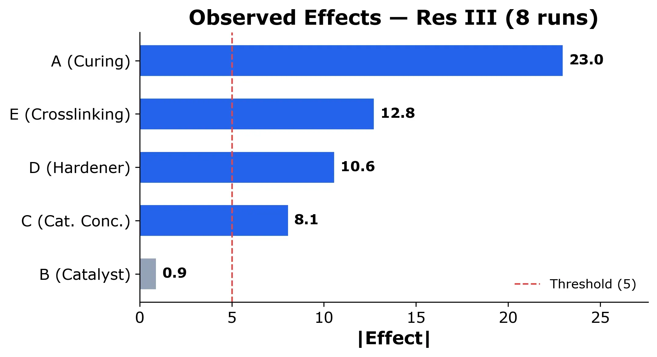
At first glance, three factors stand out. Curing Conditions (A = +23.0) is clearly the most important, followed by Crosslinking Degree (E = +12.8) and Hardener Type (D = +10.6). Catalyst Concentration (C = −8.1) also looks relevant.
But we know that Hardener Type (D) is aliased with A×E. Curing Conditions (A) and Crosslinking Degree (E) are both clearly active factors, so an A×E interaction is entirely plausible. Is Hardener Type really that important, or is the Curing Conditions × Crosslinking Degree interaction inflating the number?
We can use a foldover design to find out.
What is a Foldover Design?
A foldover design is a follow-up experiment where you run a mirror image of your original fractional factorial design. You take the original design matrix and flip the signs of one or more factors, then run those new treatment combinations.
By flipping the signs strategically, you change the confounding structure. When you combine the original and foldover data, effects that were previously tangled together become separable.
There are two main types:
- Full foldover. Flip the signs of ALL factors. If your original design is Resolution III, this increases the resolution of the combined design to Resolution IV.
- Single-factor foldover. Flip the signs of just ONE factor. This clears that factor and all its interactions from their aliases.
Let’s see how the full foldover works for our example.
Full Foldover: Flipping Everything
In a full foldover, we take our original design and reverse the sign of every factor. If a run had A = −1, B = +1, C = −1, D = +1, E = −1, the foldover run becomes A = +1, B = −1, C = +1, D = −1, E = +1.
Here’s the foldover design:
| Run | A | B | C | D | E | Pendulum Damping |
|---|---|---|---|---|---|---|
| 9 | +1 | −1 | +1 | −1 | +1 | 102.2 |
| 10 | +1 | −1 | +1 | +1 | −1 | 83.8 |
| 11 | +1 | +1 | −1 | −1 | +1 | 107.2 |
| 12 | +1 | +1 | −1 | +1 | −1 | 89.8 |
| 13 | −1 | +1 | +1 | +1 | +1 | 67.0 |
| 14 | −1 | +1 | +1 | −1 | −1 | 86.7 |
| 15 | −1 | −1 | −1 | +1 | +1 | 74.7 |
| 16 | −1 | −1 | −1 | −1 | −1 | 75.3 |
Why Does Flipping Work?
Let’s look at the algebra. Our original design has the defining relation:
I = ABC = ADE = BCDE
In the foldover, every factor changes sign. Whether a defining word survives depends on its length:
- ABC has 3 letters (odd): (−A)(−B)(−C) = (−1)³ × ABC = −ABC. The sign flips, so this word is eliminated when we combine the two halves.
- ADE has 3 letters (odd): same logic, eliminated.
- BCDE has 4 letters (even): (−B)(−C)(−D)(−E) = (−1)⁴ × BCDE = +BCDE. The sign stays, so this word survives.
The combined defining relation is just:
I = BCDE
This is a Resolution IV design. The shortest remaining word has 4 letters, which means main effects are now free of two-way interactions. The confounding between Hardener Type (D) and A×E is broken.
Deep Dive: A full foldover eliminates all odd-length words from the defining relation. Since Resolution III means the shortest word has 3 letters (odd), a full foldover of a Resolution III design always produces a Resolution IV combined design. Even-length words survive, so some confounding between two-way interactions remains, but the critical main-effect ambiguity is resolved.
Important consequence: for Resolution IV designs (where the shortest word has 4 letters, all even), a full foldover does not help. Every word has even length, so (−1)⁴ = +1 and all words survive unchanged. You’d simply duplicate your original runs in reverse order without gaining any new information. In that case, a single-factor foldover is needed instead (more on this below).
The Combined Design
When we put the original and foldover runs together, we get 16 runs. With five factors, 16 runs gives us a 2⁵⁻¹ half-fraction. This isn’t a full factorial (that would require 32 runs), but it’s a big improvement: all main effects are now estimable independently of any two-way interaction.
Two-way interactions are still partially confounded with each other. The surviving word I = BCDE means, for example, that B×C is aliased with D×E, and B×D is aliased with C×E. But that’s a far less dangerous kind of confounding. You can usually figure out which interaction is active based on which main effects are large.
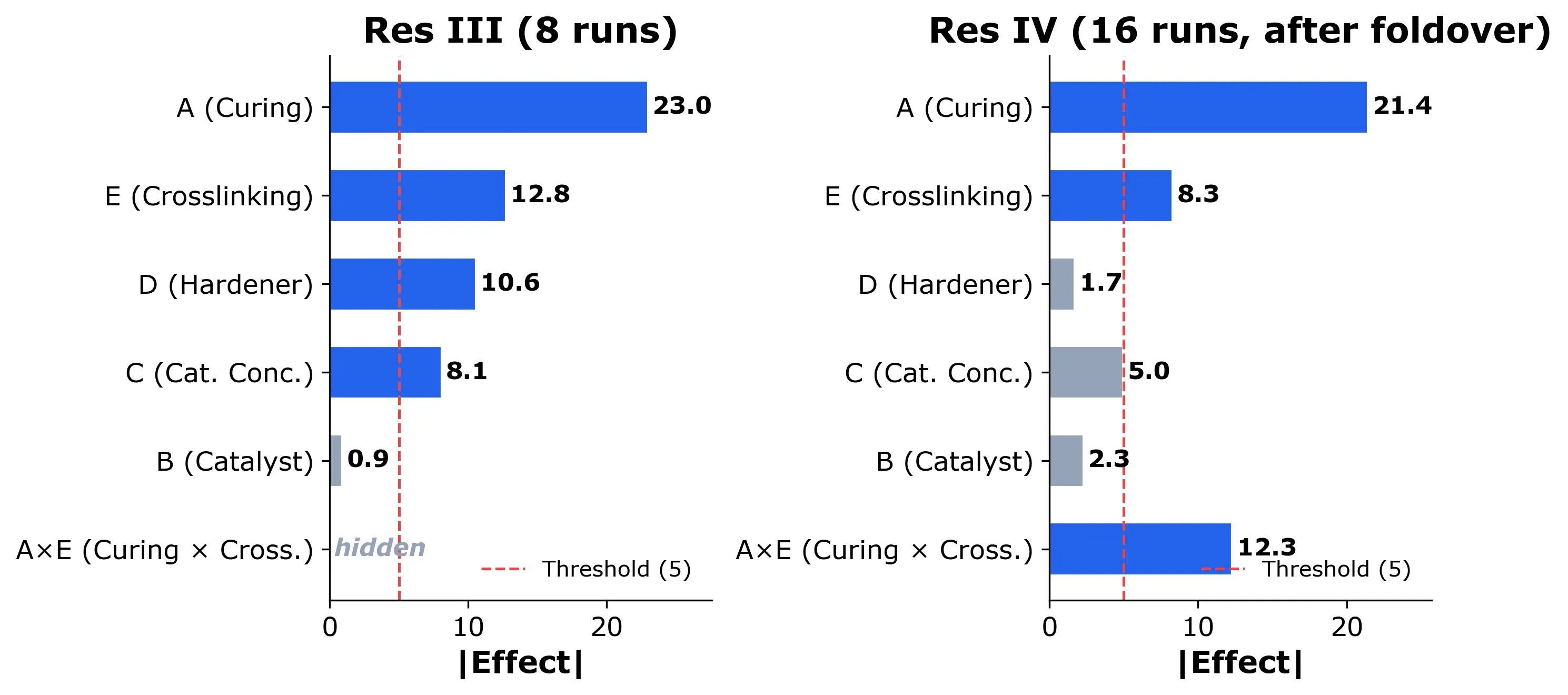
Here are the resolved effects from the combined 16-run design:
| Effect | Fractional (8 runs) | Combined (16 runs) |
|---|---|---|
| A | +23.0 | +21.4 |
| B | +0.9 | +2.3 |
| C | −8.1 | −5.0 |
| D | +10.6 | −1.7 |
| E | +12.8 | +8.3 |
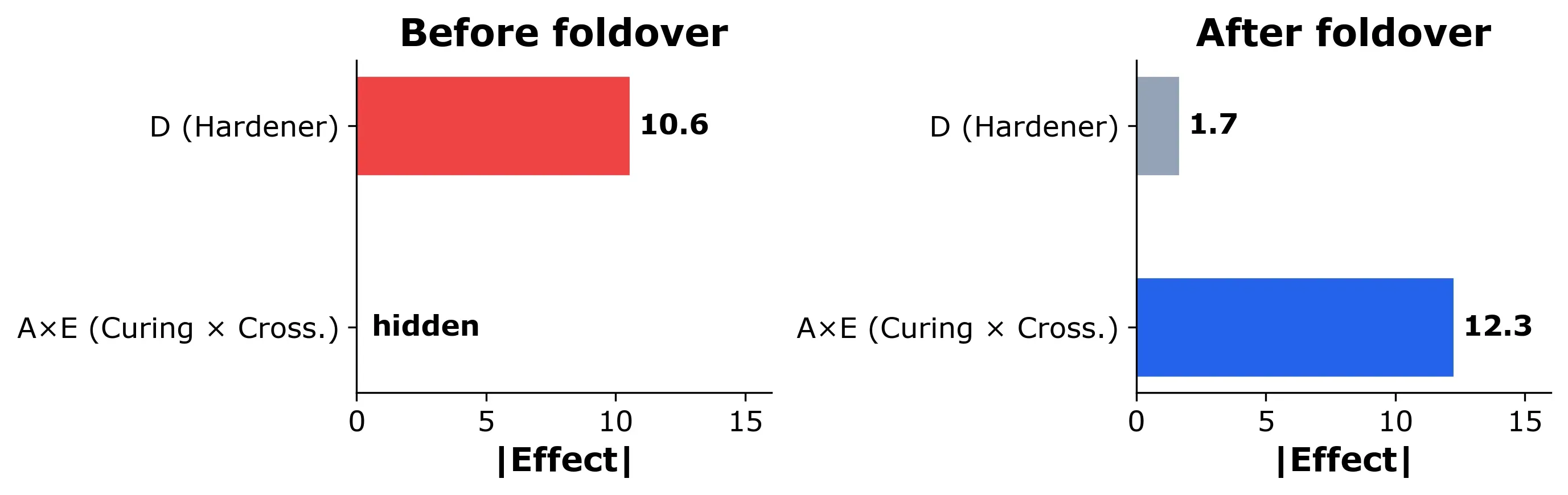
| A×E | (hidden in D) | +12.3 |
Look at Hardener Type (D). Its resolved effect is −1.7, essentially negligible. The +10.6 we observed in the fractional design was almost entirely the A×E interaction (Curing Conditions × Crosslinking Degree) showing up as a Hardener Type effect. Without the foldover, we would have concluded that Hardener Type is a critical factor when it’s actually one of the least important ones.
Curing Conditions (A) and Crosslinking Degree (E) were essentially correct in the original fractional design. Their confounded partners turned out to be small, so the estimates weren’t distorted much. Catalyst Concentration (C) was somewhat inflated by the A×B interaction: the fractional showed −8.1, while the resolved value is −5.0.
What the foldover actually uncovered is the A×E interaction at +12.3.
Single-Factor Foldover: Targeted De-Aliasing
A single-factor foldover flips the signs of only one factor. This de-aliases that factor’s main effect and all interactions involving that factor from their confounded partners.
A concrete example: flipping only Hardener Type (D)
Let’s see what would have happened if we had used a single-factor foldover instead of a full foldover in our coating example. Suppose we only wanted to resolve the D + A×E alias. We’d take the original 8 runs and flip only the D column:
| Run | A | B | C | D | E | Pendulum Damping |
|---|---|---|---|---|---|---|
| 1’ | −1 | +1 | −1 | −1 | −1 | 74.8 |
| 2’ | −1 | +1 | −1 | +1 | +1 | 76.0 |
| 3’ | −1 | −1 | +1 | −1 | −1 | 61.2 |
| 4’ | −1 | −1 | +1 | +1 | +1 | 65.5 |
| 5’ | +1 | −1 | −1 | +1 | −1 | 93.5 |
| 6’ | +1 | −1 | −1 | −1 | +1 | 106.3 |
| 7’ | +1 | +1 | +1 | +1 | −1 | 88.8 |
| 8’ | +1 | +1 | +1 | −1 | +1 | 109.3 |
In the original design, D = A×E by construction. So every time we computed the “D effect,” we were actually measuring D + A×E together. In the foldover with D flipped, D now has the opposite sign of A×E (since A and E are unchanged). This means the D column now measures D − A×E.
Here’s the separation:
- Original block: D effect = D + A×E = +10.6
- Foldover block: D effect = D − A×E = −7.0
- Pure D = (10.6 + (−7.0)) / 2 = +1.8
- Pure A×E = (10.6 − (−7.0)) / 2 = +8.8
The single-factor foldover correctly identifies Hardener Type (D) as negligible (+1.8) and the A×E interaction as the true driver (+8.8). The exact values differ slightly from the full foldover estimates (D = −1.7, A×E = +12.3) because each approach uses a different subset of 16 runs from the full 32-run factorial. But both reach the same qualitative conclusion: Hardener Type doesn’t matter, and the Curing Conditions × Crosslinking Degree interaction does.
What remains aliased?
Flipping D eliminates the word ADE from the defining relation (it contains D, so the sign flips). But ABC does not contain D, so it survives. The combined design’s defining relation is:
I = ABC
This means A is still aliased with B×C, B with A×C, and C with A×B. The combined design is still Resolution III for factors A, B, and C — only Hardener Type and its interactions are cleanly resolved.
Why the full foldover was the better choice here
In our coating experiment, Hardener Type + A×E was the most critical alias, but it wasn’t the only one worth investigating. Curing Conditions (A = +23.0) was aliased with B×C and D×E. Crosslinking Degree (E = +12.8) was aliased with A×D. Even Catalyst Concentration (C = −8.1) was aliased with A×B.
A full foldover resolved all main effects from their two-way interaction aliases in a single step. The single-factor approach would only have cleared Hardener Type, leaving potential ambiguity in the other estimates.
Note: for half-fraction designs (like a 2⁴⁻¹), this limitation disappears. A single-factor foldover of a half-fraction generates the complementary half-fraction, giving you the complete full factorial. Since the defining relation has only one word, flipping any factor in it eliminates that word entirely, clearing all effects — not just those involving the flipped factor.
Key Takeaways
A foldover design is a follow-up experiment that resolves confounding by running a mirror image of your original fractional factorial. By flipping the signs of factors, you change the alias structure so that previously entangled effects become separable.
A full foldover (flipping all factors) eliminates all odd-length words from the defining relation. For a Resolution III design, this means main effects become clear of two-way interactions.
A single-factor foldover is more targeted. It clears one specific factor and its interactions but leaves other confounding intact, unless you’re working with a half-fraction, in which one case any single-factor foldover completes the full factorial and resolves everything.