
All-Subset Regression
In How to Perform ANOVA, we built a model for our filtration rate experiment using backward elimination. We started with all terms, checked p-values, removed the weakest, refitted, and repeated until only significant terms remained. It worked, and we ended up with a good model.
But the process involved decisions at every step. Which term do you remove first? Do you start from main effects up or from the full model down? Could a different path through the elimination steps lead to a different final model?
All-subset regression takes a completely different approach. Instead of building the model step by step, it evaluates every possible combination of your candidate terms and picks the one that fits best. No iterative decisions, no path dependence, just a systematic search through all options.
What is all-subset regression?
The idea is simple. You have a set of candidate model terms: main effects, interactions, whatever you want to include. All-subset regression works through four steps:
- Enumerate every possible subset of those terms (from single-term models up to the full model)
- Fit a regression model for each subset
- Evaluate each model using a quality metric
- Select the best one
Each model is fitted independently. The result for the subset {T, RPM, T×RPM} has nothing to do with what was found for {T, RPM} or {T, CoF, RPM}. There is no path through model space. Every subset stands on its own merits.
This is the key difference from backward elimination or forward selection. Those methods condition each step on the previous selection. Change the removal order, and you might end up at a different final model. All-subset regression doesn’t have that problem. Whatever model wins, it wins because it is the best among all candidates.
How many models are we talking about?
For our filtration rate experiment, we have four factors (T, P, CoF, RPM) and six possible two-factor interactions (T×P, T×CoF, T×RPM, P×CoF, P×RPM, CoF×RPM). That’s 10 candidate terms in total. The number of possible non-empty subsets is 2^10 − 1 = 1,023 models.
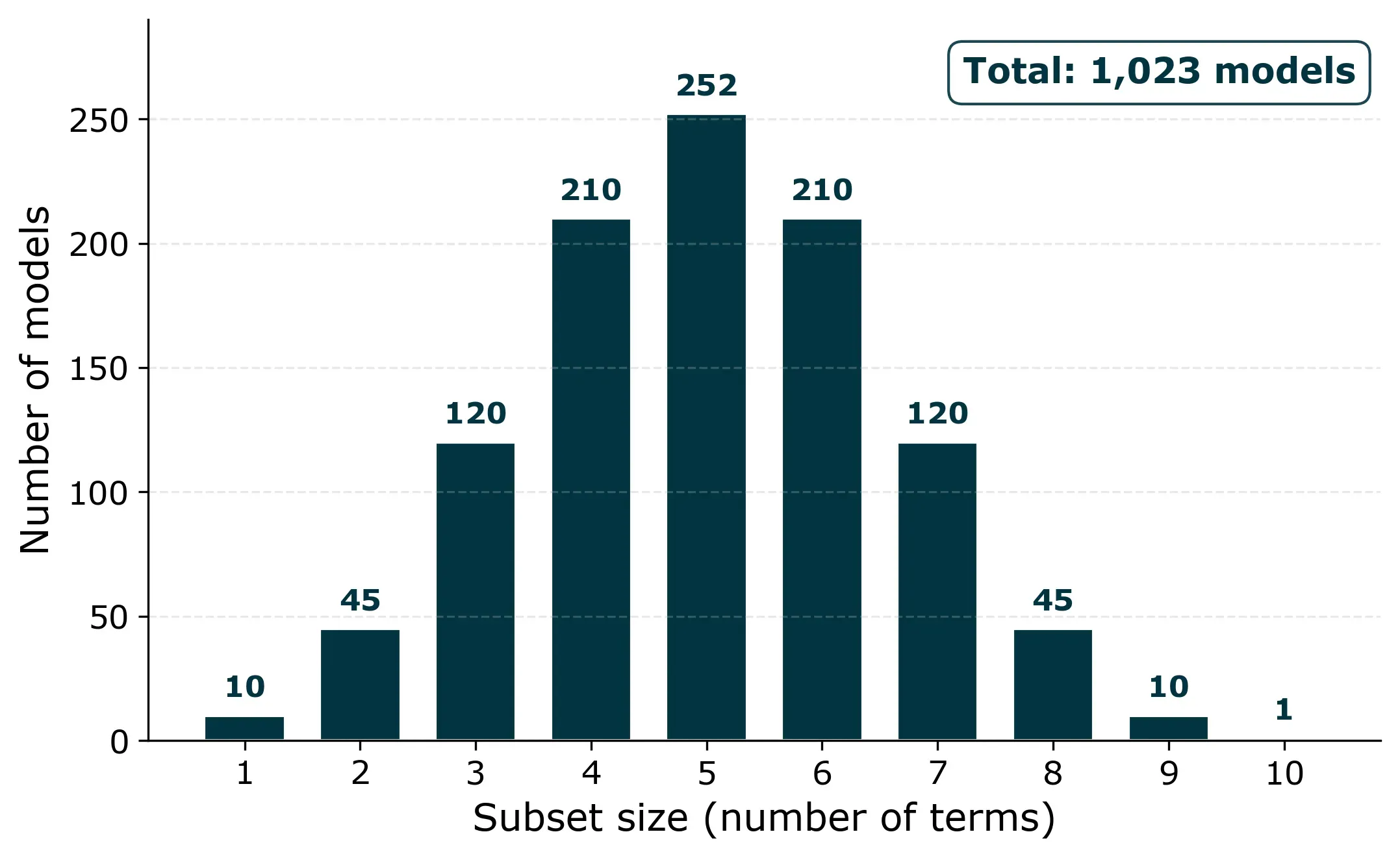
That sounds like a lot, but a computer can fit all of them in under a second. For problems with up to about 10 to 12 candidate terms, all-subset regression is perfectly feasible.
Why not just use R²?
Since we’re comparing models of different sizes, we need a metric that accounts for complexity. Plain R² always increases when you add more terms, even useless ones. A 10-term model will always have a higher R² than a 5-term model, regardless of whether those extra terms contribute anything real.
Two metrics handle this well:
Adjusted R² penalizes the number of terms. Unlike plain R², it can actually decrease when you add a factor that doesn’t contribute enough:
Adj. R² = 1 − (1 − R²) × (n − 1) / (n − p − 1)
where n is the number of observations and p is the number of terms.
BIC (Bayesian Information Criterion) penalizes complexity more aggressively. Lower values are better:
BIC = n × ln(RSS / n) + k × ln(n)
where RSS is the residual sum of squares and k is the total number of parameters (terms + intercept).
Applying it to the filtration rate data
Let’s apply all-subset regression to the same dataset we used in the ANOVA post: a 2^4 full factorial design with four factors (Temperature, Pressure, Concentration of Formaldehyde, and Stirring Rate) and 16 runs.
We include all four main effects and all six two-factor interactions as candidates. That gives us 1,023 models to evaluate. For each one, we fit an OLS regression and compute adjusted R² and BIC.
Adjusted R² as quality metric
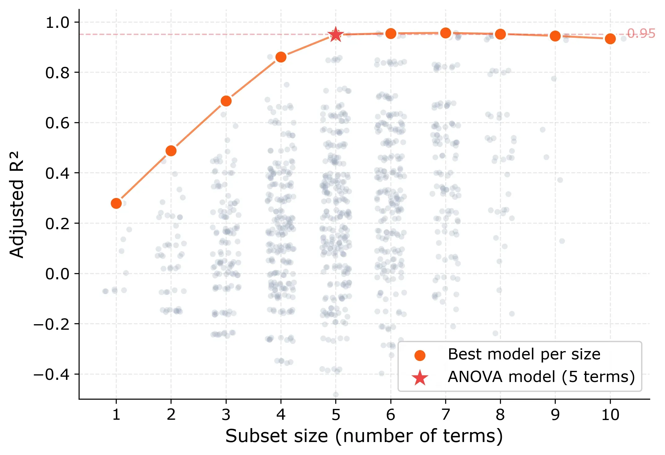
The pattern tells a clear story. Models with only main effects, without any two-way interactions top out at an adjusted R² of 0.43. So less than half the variation is explained. Interactions are clearly needed.
The big jump happens between size 4 and 5. The best 4-term model reaches 0.86, while the best 5-term model hits 0.95. After that, adding more terms barely changes anything. The curve flattens into a plateau from size 5 onward.
Here are the best models at each size:
| Size | Best subset | Adj. R² | BIC |
|---|---|---|---|
| 1 | T | 0.278 | 93.3 |
| 2 | T, T×CoF | 0.487 | 89.4 |
| 3 | T, T×CoF, T×RPM | 0.686 | 83.1 |
| 4 | T, RPM, T×CoF, T×RPM | 0.861 | 71.5 |
| 5 | T, CoF, RPM, T×CoF, T×RPM | 0.949 | 56.7 |
| 6 | T, P, CoF, RPM, T×CoF, T×RPM | 0.955 | 55.9 |
Notice what happens at size 5: the model includes T, CoF, RPM, T×CoF, and T×RPM. That’s exactly the model we found through ANOVA backward elimination.
The 6-term model adds Pressure (P) and squeezes out a tiny bit more adjusted R² (0.955 vs 0.949). But P’s coefficient is only 1.56, compared to 10.81 for T and 7.31 for RPM. That small contribution is more likely noise than a real physical effect.
BIC as quality metric
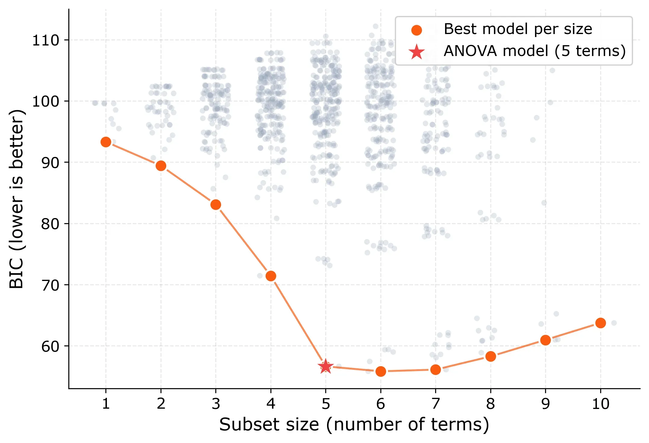
BIC shows the same story more sharply. It drops steadily from size 1 to size 5, then flattens. The global BIC minimum is actually at size 6 (55.9 vs. 56.7), but the difference is small. BIC differences below 2 are generally considered negligible.
The 5-term model sits right at the elbow: the point where adding more terms stops providing meaningful improvement. This “elbow” pattern is the signature you’re looking for in all-subset regression. It tells you: this is the right model size.
Comparison with ANOVA
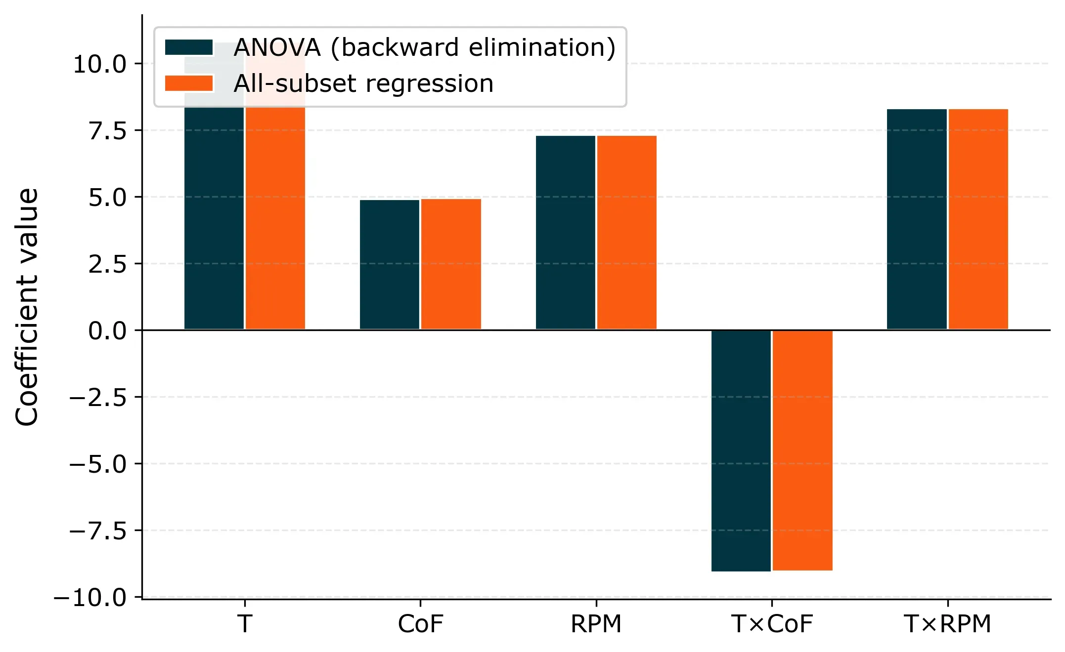
Both methods arrive at the same final model:
Filtration Rate = 70.1 + 10.8·T + 4.9·CoF + 7.3·RPM − 9.1·(T×CoF) + 8.3·(T×RPM)
The coefficients are identical, because the underlying model is the same.
So if both methods give the same answer, why bother with all-subset regression?
The difference is in how they get there.
ANOVA backward elimination required multiple rounds. In the ANOVA post, we started with 15 terms (4 main effects + 6 two-way + 4 three-way + 1 four-way interaction), removed T×CoF×RPM first (highest p-value among three-way interactions), then refitted, removed the next weakest, refitted again, and so on. Each removal changed the p-values of the remaining terms, so the order mattered. Forward selection required similar judgment calls about which terms to try adding.
All-subset regression evaluates all 1,023 models at once and selects the winner directly. No intermediate decisions, no removal order, no judgment calls. The same data always produces the same result.
There’s also a fundamental difference in what drives the decision. ANOVA decides whether a term stays or goes based on its p-value relative to a threshold, usually 0.05. But that threshold is arbitrary. A term with p = 0.06 gets removed, one with p = 0.04 stays, even though the practical difference between those two values is negligible. With noisy data or small sample sizes, p-values become unstable: rerun the same experiment and a “significant” term might flip to non-significant or vice versa. All-subset regression doesn’t use p-values at all. It compares overall model fit using adjusted R² and BIC, which measure how well the entire model explains the data rather than testing each term in isolation.
On top of that, the adjusted R² and BIC curves give you a built-in diagnostic. If the best model at any size has a low adjusted R² and there’s no elbow, that’s a strong signal that something is missing from your candidate pool, perhaps an interaction you didn’t include. ANOVA doesn’t give you that kind of feedback as directly.
When to use it
If your candidate pool has roughly up to 10 to 12 terms, I’d recommend using all-subset regression as your default approach. It’s more objective than stepwise methods, it doesn’t depend on arbitrary p-value thresholds, and the elbow diagnostic comes for free. With 10 terms you’re evaluating about 1,000 models. With 12, about 4,000. A modern computer handles that without breaking a sweat.
The only real limitation is computational. Once you go beyond about 15 terms, the number of subsets grows into the hundreds of thousands and becomes impractical. At that point, methods like LASSO or stepwise regression are more appropriate. But for typical factorial experiments with 4 to 8 factors and their interactions, all-subset regression is the cleaner tool.
Key takeaways
All-subset regression evaluates every possible combination of your candidate terms and selects the best model directly. No iterative steps, no path dependence, no reliance on p-value thresholds.
Use adjusted R² or BIC to compare models of different sizes, never plain R². BIC is typically more decisive at pinpointing the right model size.
Look for the “elbow” in the metric curves. A sharp improvement followed by a plateau tells you the model has captured the essential structure of your data. A flat curve with low adjusted R² tells you something is missing.
For the filtration rate experiment, all-subset regression and ANOVA backward elimination found the same 5-term model with the same coefficients. The advantage of all-subset regression is objectivity: the data decides which model wins, not the order in which you happen to test terms or where you draw a significance line.