I recently showed how to use BayBE and NEXTorch for Bayesian Optimization. Now let’s look at the third Python package: BoFire.

BoFire (Bayesian Optimization Framework Intended for Real Experiments) is a Python library that according to the documentation “is actively used by hundreds of users across leading organizations such as Agilent, BASF, Bayer, Boehringer Ingelheim and Evonik”. It’s built on BoTorch and designed specifically for real-world experimental challenges in chemistry and materials science. In this blog post I’ll cover the basics to get you started. Check out the BoFire documentation for more details, and I’ve created an AI agent that can help you with BoFire questions and write code for you.

Like BayBE, BoFire accepts chemical descriptors as inputs for molecules and is actively maintained.

Let’s look at how BoFire works.

The BoFire workflow

BoFire separates what you want to optimize (the data model) from how to optimize it (the strategy). This clean separation makes it easy to swap algorithms or add constraints without rewriting your code.

Here’s the typical workflow:

1. Define the domain (inputs, outputs, constraints)
2. Choose a strategy for generating experiments
3. Run the optimization loop: ask → experiment → tell
4. Analyze results

I’ll walk through a concrete example using the same objective function from my previous tutorials so you can compare the frameworks.

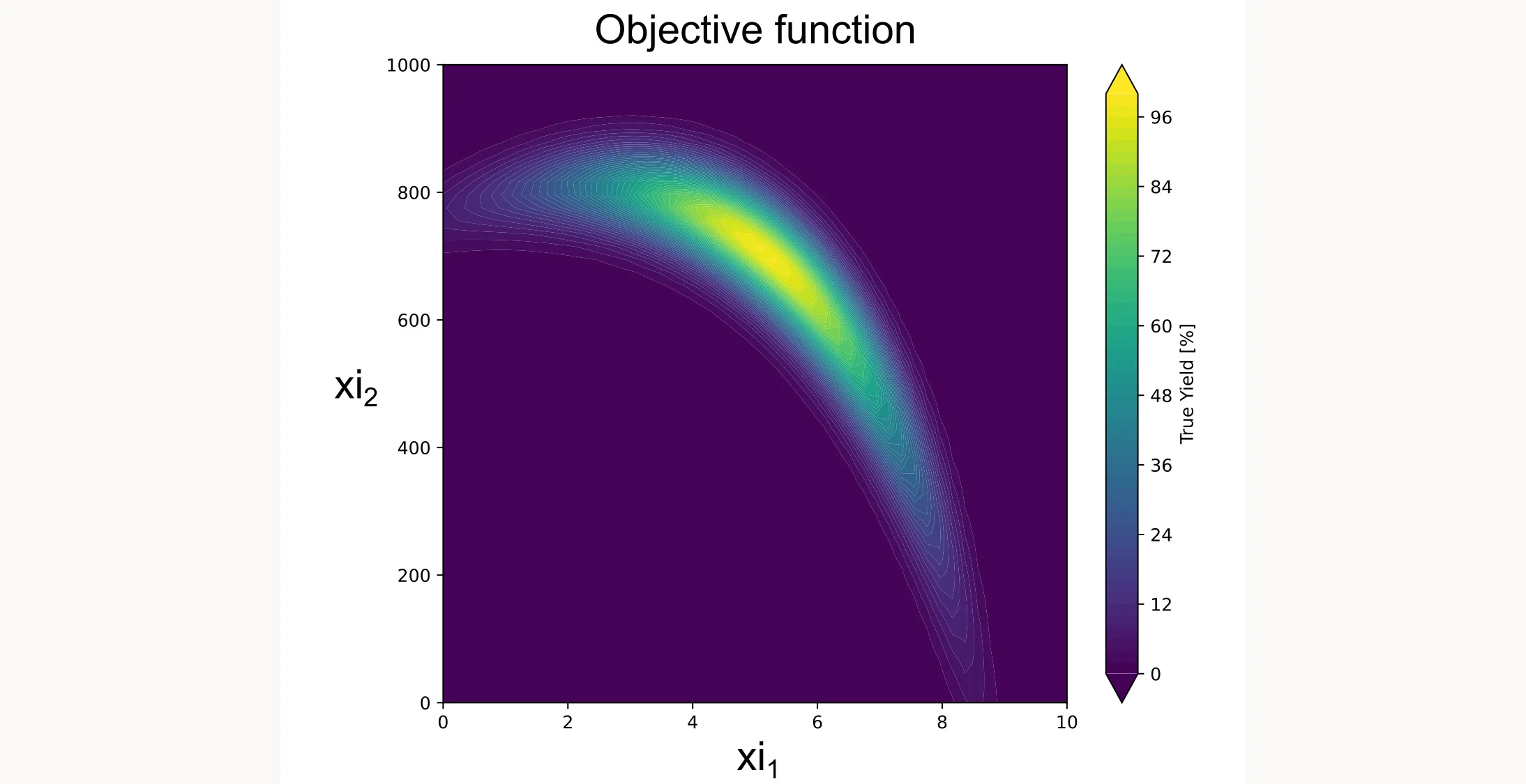
Step 1: Define the objective function

import numpy as np
import pandas as pd
import matplotlib.pyplot as plt

import bofire.strategies.api as strategies
from bofire.data_models.features.api import ContinuousInput, ContinuousOutput
from bofire.data_models.objectives.api import MaximizeObjective
from bofire.data_models.domain.api import Domain, Inputs
from bofire.data_models.strategies.api import SoboStrategy, RandomStrategy, StepwiseStrategy, Step
from bofire.data_models.strategies.api import NumberOfExperimentsCondition, AlwaysTrueCondition
from bofire.data_models.acquisition_functions.api import qLogEI
from bofire.data_models.enum import SamplingMethodEnum

def yield_fn(xi1, xi2):
    """
    Objective function that simulates a yield optimization problem.
    """
    xi1, xi2 = float(xi1), float(xi2)
    x1_t, x2_t = 3 * xi1 - 15, xi2 / 50.0 - 13
    c, s = np.cos(0.5), np.sin(0.5)
    x1_r = c * x1_t - s * x2_t
    x2_r = s * x1_t + c * x2_t
    y = np.exp(-x1_r**2 / 80.0 - 0.5 * (x2_r + 0.03 * x1_r**2 - 40 * 0.03)**2)
    return 100.0 * y

Here’s what it looks like:

Step 2: Define the domain

In BoFire, the domain defines your optimization problem: what inputs you can control, what outputs you want to optimize, and any constraints. Here’s how you define a simple domain with two continuous inputs:

domain = Domain.from_lists(
    inputs=[
        ContinuousInput(key="xi1", bounds=(0, 10)),
        ContinuousInput(key="xi2", bounds=(0, 1000)),
    ],
    outputs=[
        ContinuousOutput(key="yield", objective=MaximizeObjective()),
    ],
)

In your real application, xi1 and xi2 might be temperature, concentration, reaction time, or any other continuous variable you can control.

Available input types

BoFire supports a wide range of input types for different experimental scenarios:

Input Type	Use Case	Example
ContinuousInput	Continuous numeric variables	Temperature (20-100°C), concentration (0-1 M)
DiscreteInput	Finite numeric values	Stirring speeds: 100, 200, 300 rpm
CategoricalInput	Categorical options without descriptors	Solvent: water, ethanol, acetone
CategoricalDescriptorInput	Categorical options with numeric descriptors	Solvents with polarity, viscosity values
ContinuousDescriptorInput	Continuous inputs with descriptors	(Experimental support)
MolecularInput	SMILES strings for molecular optimization	Drug candidates, catalyst ligands

The descriptor-based inputs (CategoricalDescriptorInput) are particularly powerful. They let the optimizer learn from molecular properties rather than treating each molecule as an independent category.

Step 3: Choose your strategy

Next you need to define the optimization strategy. BoFire gives you two main approaches for structuring your optimization:

Option A: StepwiseStrategy

StepwiseStrategy automatically handles the transition from initial exploration to Bayesian optimization. You first gather information about the search space through random sampling or a DoE approach, then switch to Bayesian optimization once you have enough initial data.

strategy_data = StepwiseStrategy(
    domain=domain,
    steps=[
        Step(
            strategy_data=RandomStrategy(domain=domain),
            condition=NumberOfExperimentsCondition(n_experiments=3)
        ),
        Step(
            strategy_data=SoboStrategy(domain=domain, acquisition_function=qLogEI()),
            condition=AlwaysTrueCondition()
        )
    ]
)
strategy = strategies.map(strategy_data)

This configuration:

• Uses RandomStrategy for the first 3 experiments (exploration phase)
• Switches to SoboStrategy with the qLogEI acquisition function for all subsequent experiments

The NumberOfExperimentsCondition(n_experiments=3) means “use this strategy until 3 total experiments exist,” then move to the next step.

SoboStrategy stands for Single-Objective Bayesian Optimization. It uses a Gaussian Process surrogate by default and optimizes the acquisition function to select the next experiment.

qLogEI (Log Expected Improvement) is a robust acquisition function that balances exploration and exploitation. The ‘q’ prefix means it can suggest multiple experiments in a batch.

Option B: Manual control with SoboStrategy

If you want explicit control over initial data generation (perhaps you have existing data or want to use a specific DoE design), use SoboStrategy directly and provide your own initial data through strategy.tell:

# Create the Bayesian Optimization strategy
strategy_data = SoboStrategy(
    domain=domain,
    acquisition_function=qLogEI(),
)
strategy = strategies.map(strategy_data)

# Generate initial data using Latin Hypercube Sampling
initial_candidates = domain.inputs.sample(n=3, method=SamplingMethodEnum.LHS)
initial_experiments = initial_candidates.copy()
initial_experiments["yield"] = initial_candidates.apply(
    lambda row: yield_fn(row["xi1"], row["xi2"]), axis=1
)

# Feed initial data to the strategy
strategy.tell(experiments=initial_experiments)

BoFire supports for example Latin Hypercube Sampling (SamplingMethodEnum.LHS) but you can use any sampling method you like, even custom ones.

Step 4: Run the optimization loop

With either approach, the optimization loop follows the same pattern. The only difference is that with option B you already “told” the strategy about your initial data. Therefore we only need to run the loop for 12 iterations (12 additional experiments to the 3 initial experiments):

print("Starting BoFire Optimization...")
for i in range(12):
    # Ask for the next candidate(s)
    candidates = strategy.ask(candidate_count=1)

    # Evaluate the objective function (in real life: run your experiment)
    xi1 = candidates["xi1"].iloc[0]
    xi2 = candidates["xi2"].iloc[0]
    y = yield_fn(xi1, xi2)

    # Create experiment DataFrame with results
    experiments = candidates.copy()
    experiments["yield"] = y

    # Tell the strategy about the new result
    strategy.tell(experiments=experiments)

    print(f"Trial {i+1:02d}: xi1={xi1:6.2f}, xi2={xi2:7.2f} | Yield = {y:6.2f}%")

The loop is straightforward:

1. ask() suggests the next experiment based on all previous data
2. You run the experiment (here, evaluating yield_fn)
3. tell() updates the internal model with the new result

In a real lab setting, you wouldn’t have a for loop. You’d call ask() when you’re ready for the next experiment, run it in the lab (which might take hours or days), then call tell() with your results. You are the for loop.

Step 5: Extract and visualize results

After running the optimization loop for a total of 15 iterations (3 initial experiments + 12 additional experiments), we can extract the results. In practice, you would do this after each iteration of the loop:

all_experiments = strategy.experiments
best_idx = all_experiments["yield"].idxmax()
print(f"Best Yield: {all_experiments.loc[best_idx, 'yield']:.2f}%")
print(f"Optimal Parameters: xi1={all_experiments.loc[best_idx, 'xi1']:.2f}, "
      f"xi2={all_experiments.loc[best_idx, 'xi2']:.2f}")

Note: Unlike NexTorch, BoFire doesn’t provide a built-in way for creating plots. You have to do this yourself (or ask an AI agent to do it for you).

Cumulative best plot

This shows how the best observed yield improves over the course of optimization:

yield_values = all_experiments["yield"].values
cum_max_values = np.maximum.accumulate(yield_values)

plt.figure(figsize=(10, 6))
plt.scatter(range(1, len(yield_values) + 1), yield_values,
            color='#E63946', alpha=0.4, s=80, label='Individual Trials')
plt.plot(range(1, len(cum_max_values) + 1), cum_max_values,
         color='#E63946', marker='s', linewidth=2, label='Cumulative Best')
plt.title("Optimization Progress with BoFire", fontsize=14)
plt.xlabel("Trial Number", fontsize=12)
plt.ylabel("Yield [%]", fontsize=12)
plt.ylim(0, 105)
plt.grid(True, linestyle='--', alpha=0.6)
plt.legend(loc='lower right')
plt.tight_layout()
plt.show()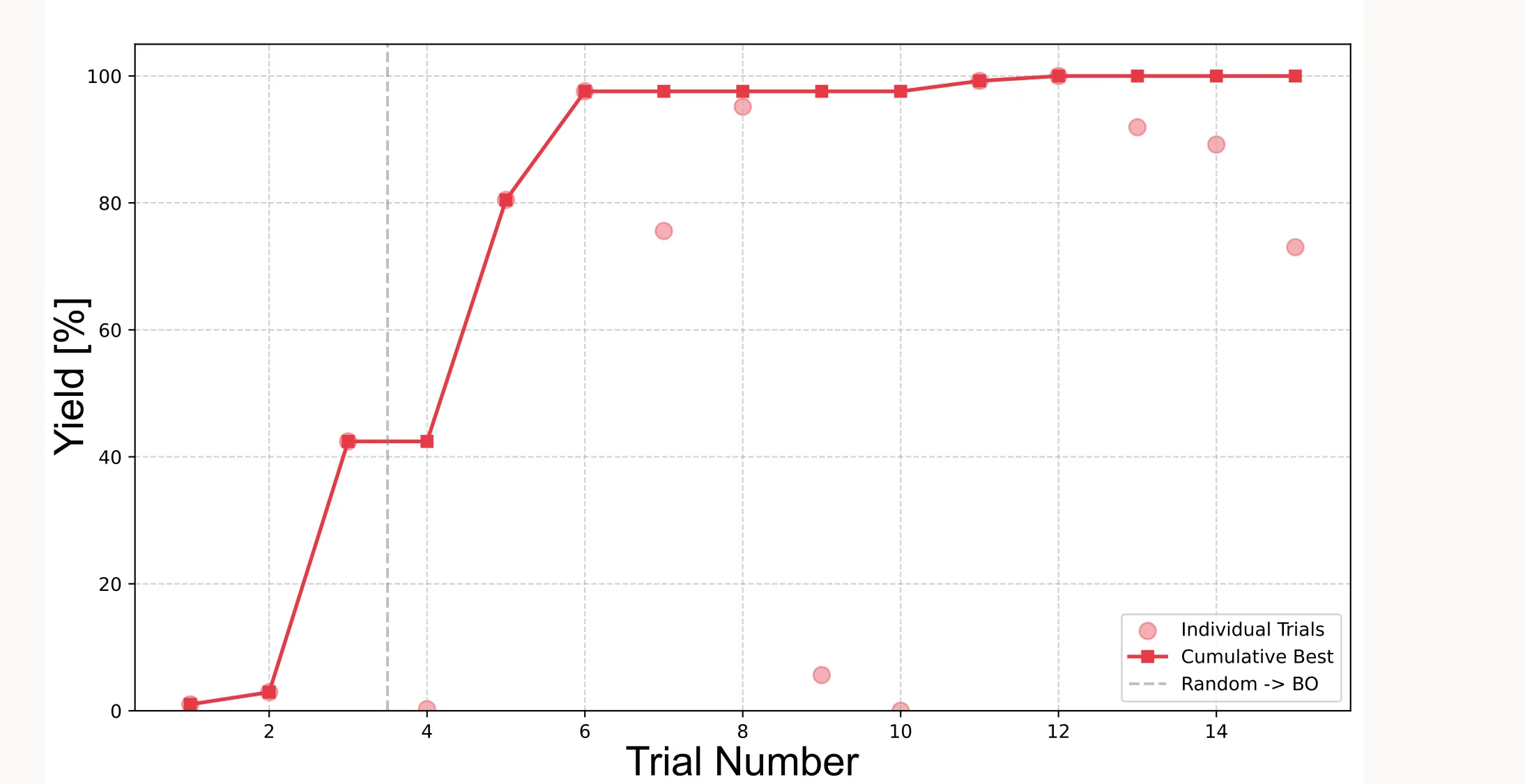

Important: Because the initial points are sampled randomly (or quasi-randomly with LHS), results will vary between runs. Sometimes the algorithm finds the optimum faster, sometimes slower. It very much depends on how good the initial points are.

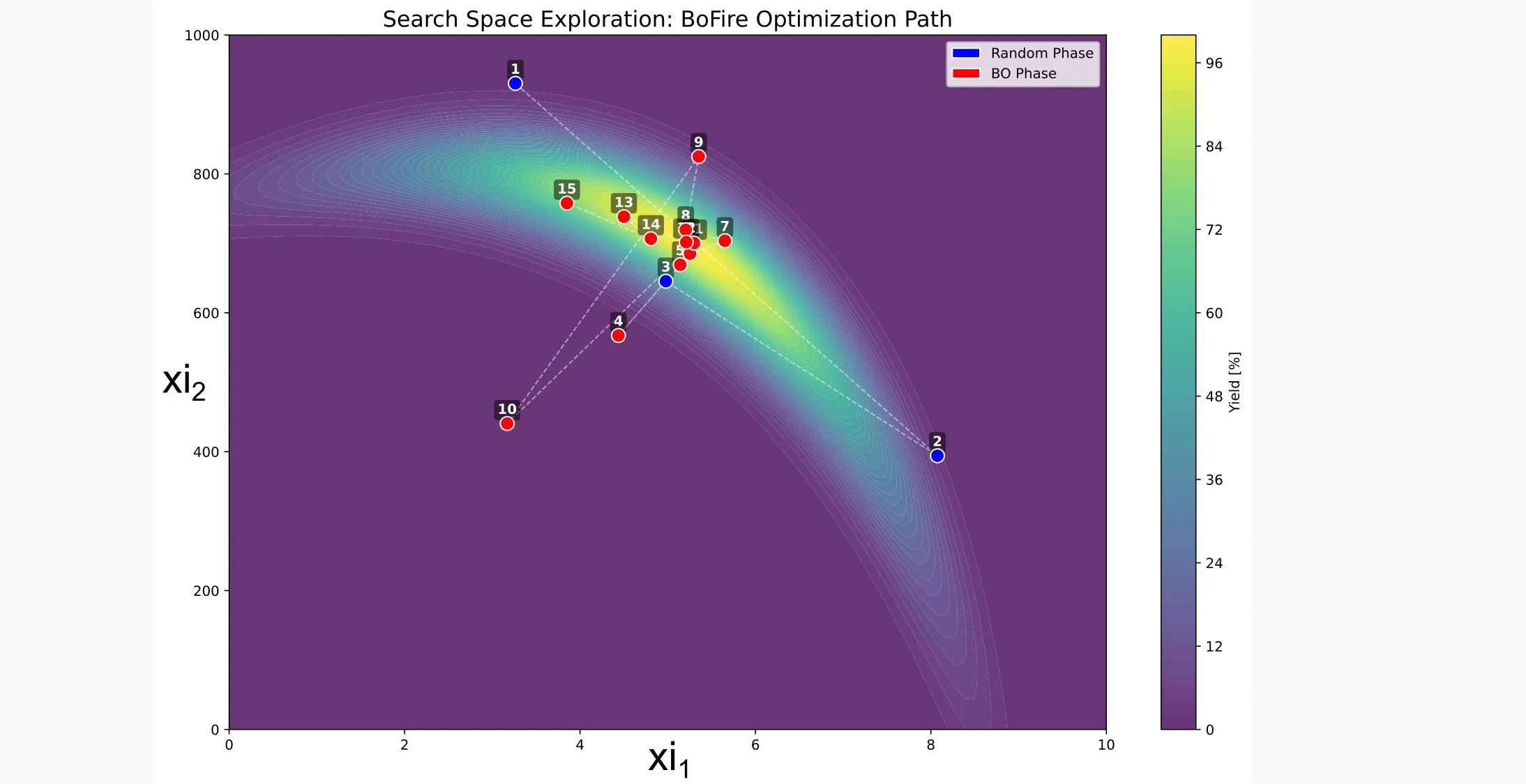
Search space coverage

You can also visualize which points were sampled during optimization:

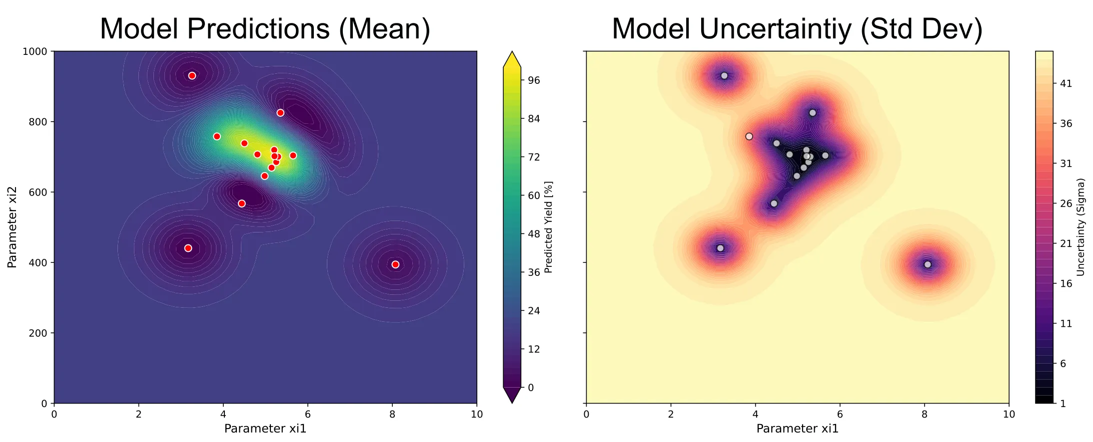
Surrogate model and uncertainty

As well as the predictions of the surrogate model and its uncertainty:

The full code is available in my GitHub repository.

If you have any questions or comments, reach out through LinkedIn or the contact form on the website.

Up next

<< Getting Started with Bayesian Optimization (NEXTorch) >>

<< Getting Started with Bayesian Optimization (BayBE) >>