Residual Analysis

You’ve conducted a DoE, visualized the results, and used ANOVA to create a model for decision making. But how good will the decisions be based on your model? You need to validate it first.

Visual Comparison

One of the simplest forms of model validation is visually comparing predicted values to measured values. This method offers a quick impression of whether the model is reasonable. Take a look at the plots below. Although the measured points may seem to deviate significantly from the red line, the good fit effectively captures the overall trend of the data. This is not the case for the bad fit, where we clearly see a curvature that the model fails to account for.

Good vs Bad Model Fit Comparison

Figure 1: Visual comparison of model fits. Left: Good model fit showing data points following the predicted trend line. Right: Poor model fit where the linear model fails to capture the curved relationship in the data.

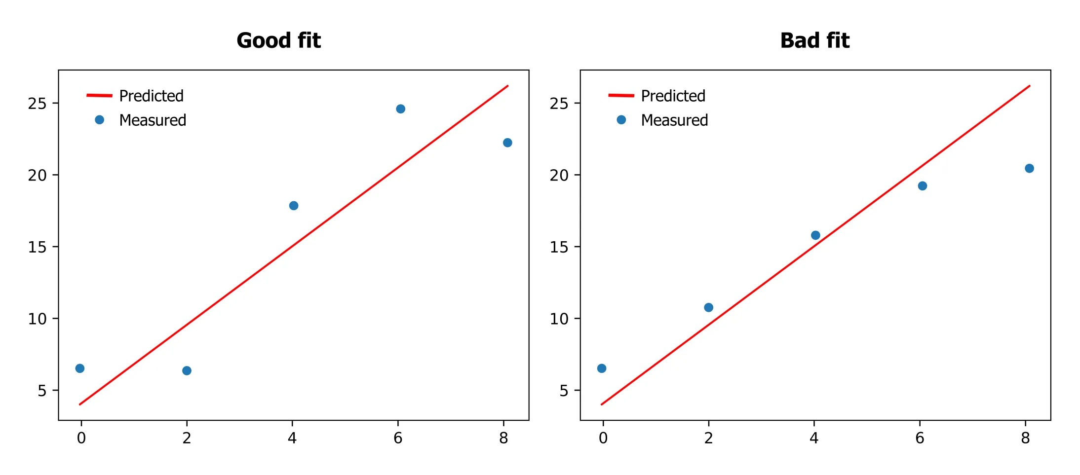
However, as the number of factors and response variables increases, visual comparisons become challenging. Residual analysis offers a more systematic approach.

What are residuals?

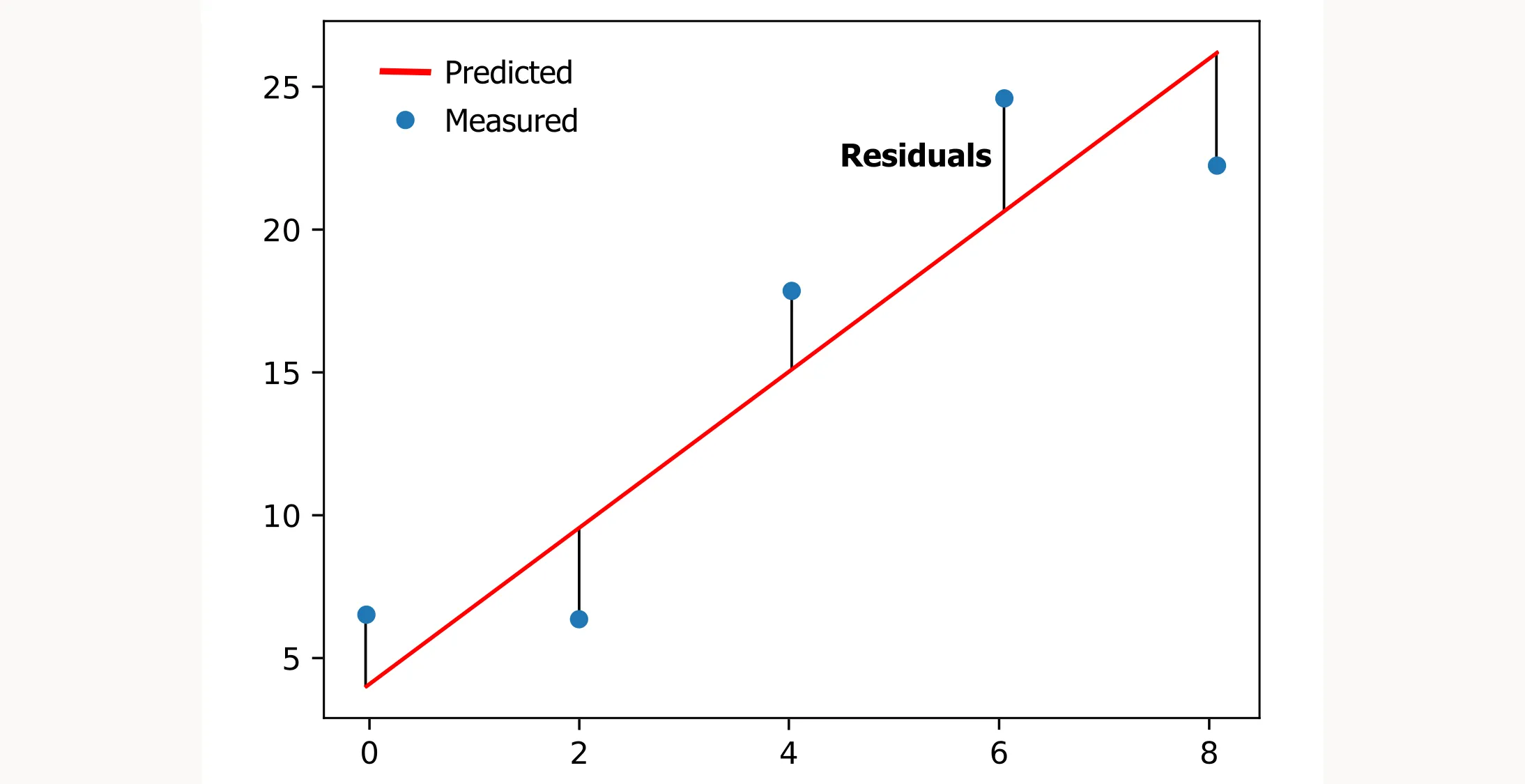
Residuals are the differences between the observed values and the values predicted by the model. They provide insight into the model’s accuracy.

Residuals Illustration

Figure 2: Residuals are the vertical distances between observed data points (blue dots) and the predicted values (red line). Positive residuals occur when observed values are above the predicted line, negative residuals when below.

Residual Sum of Squares

One way to assess the quality of your model is by calculating the residual sum of squares (RSS). As the name suggests, RSS is the sum of the squared residuals. Squaring the residuals ensures that both positive and negative deviations are accounted for, preventing them from canceling each other out. Generally, the smaller the RSS, the better the model.

RSS = Σ (y_i - ŷ_i)²

where y_i is the observed value and ŷ_i is the predicted value.

Temperature	Concentration	Pressure	Measured Result (Y)	Predicted Result (Ŷ)	Residual (Y - Ŷ)	RSS
25	0.1	1	5.0	4.8	0.2	0.04
30	0.2	1.5	6.2	6.0	0.2	0.04
35	0.3	2	7.1	7.3	-0.2	0.04
40	0.4	2.5	8.3	8.1	0.2	0.04
45	0.5	3	9.0	8.9	0.1	0.01
50	0.6	3.5	10.1	10.0	0.1	0.01

Total RSS = 0.18

One problem with the residual sum of squares (RSS) is that it is not standardized, meaning its value depends on the scale of the data and the number of data points. This makes it difficult to compare the goodness of fit across different models or datasets.

R-squared

R-squared is a better metric because it’s standardized. You might recognize this statistical measure from Excel. It ranges from 0 to 1, making it easier to interpret and compare across different models. It represents how much of the variation in the response can be explained by the tested factors. An R-squared value closer to 1 indicates a better fit, meaning the model explains more of the variance.

The formula to calculate R-squared is:

R² = 1 - (SS_res / SS_tot)

where:

SS_res is the residual sum of squares (RSS). SS_tot is the total sum of squares.

R-squared = 1: This indicates that the model explains 100% of the variance in the response variable. The predicted values perfectly match the observed data.

R-squared = 0: This indicates that the model does not explain any of the variance in the response variable. The model’s predictions are no better than the mean of the observed data.

0 < R-squared < 1: Values between 0 and 1 indicate the proportion of the variance in the dependent variable that is predictable from the independent variables. For example, an R-squared of 0.9 means that 90% of the variance in the response variable is explained by the model.

Note: R-squared increases (or stays the same) as more predictors are added and therefore does not penalize model complexity.

R-squared Interpretation

Figure 3: Visual comparison of different R-squared values: Left shows R² = 1 (perfect fit), middle shows R² = 0.9 (very good fit), and right shows R² = 0 (no fit). Higher R-squared values indicate that more variance is explained by the model.

R-squared has limitations though. It doesn’t reveal non-linearity or time-dependent effects. Residual plots can uncover these issues.

Residual Plots

Residuals vs. Predicted:

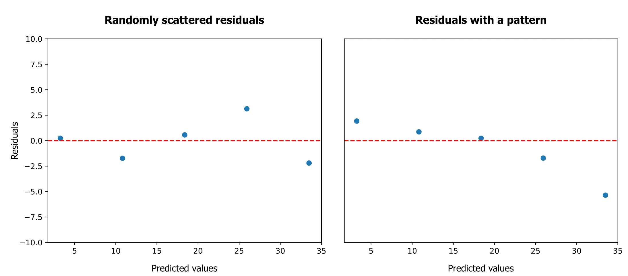
A residuals vs. predicted plot shows the residuals (errors) on the vertical axis and the predicted values on the horizontal axis. You want to see a random scatter, which indicates a good fit.

Curved pattern: suggests a missing functional form. Consider adding polynomial terms (e.g., quadratic), interactions, or applying an appropriate transformation.
Funnel/trumpet shape: indicates heteroscedasticity (non-constant variance). Consider transforming the response (log/square-root/Box–Cox) or using weighted least squares.

Residuals vs Predicted Plots

Figure 4: Examples of residuals vs predicted plots: left shows ideal random scatter (good model), right shows curved pattern.

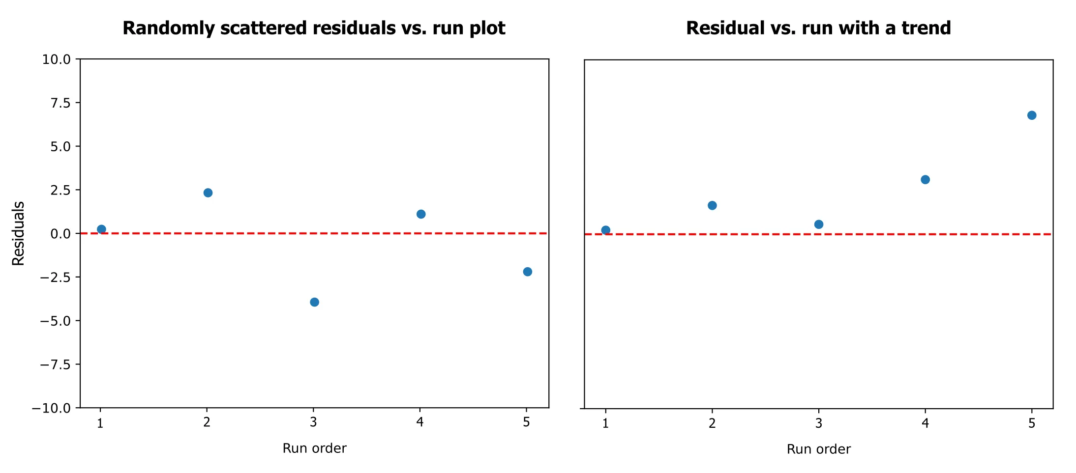
Residuals vs. Run Order:

The residuals vs. run order plot shows the residuals versus the chronological order of the experiments. Again, you want random scatter. Trends in this plot can reveal time-dependent effects like temperature changes during the experiment, equipment drift, or operator fatigue. Blocking and randomization help prevent these trends from affecting your analysis.

Residuals vs Run Order Plots

Figure 5: Examples of residuals vs run order plots: Left shows ideal random scatter with no time-dependent effects, right shows problematic trend indicating systematic changes during the experiment (e.g., equipment drift, temperature changes, or operator fatigue).

Model validation is critical for confirming the reliability of your experimental findings. Skip it, and you risk making decisions based on faulty models.