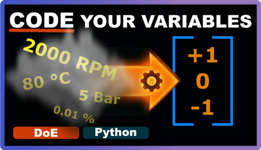
Why You Should Always Code Your Variables

Say you’re running an experiment with concentration ranging from 0.1% to 1.0% and stirring rate from 1000 to 2000 RPM. If you fit a model using these raw values, the stirring rate coefficient might be 0.02 while the concentration coefficient is 15. Does that mean concentration matters 750 times more? No. The numbers are just on different scales. Stirring rate looks tiny because you’re measuring in thousands, while concentration looks huge because you’re measuring in fractions.

Coding your variables fixes this by putting everything on the same scale, usually from -1 to +1.

A Full Example

Let’s take a look at an actual filtration rate experiment where four factors are varied:

Temperature (T): 20°C to 80°C
Pressure (P): 1 bar to 5 bar
Concentration (CoF): 0.1% to 1.0%
Stirring Rate (RPM): 1000 to 2000

Using natural units, the regression model looks like this:

$\text{Filtration Rate} = 21.73 + 0.36(T) + 0.78(P) + 10.97(CoF) + 0.015(RPM)$

At first glance, concentration dominates with a coefficient of 10.97, while stirring rate appears irrelevant at 0.015. That’s a 730x difference. Same fort the other factors. But this is misleading. The coefficients reflect the measurement scales, not the actual importance. A 1-unit change in RPM (from 1000 to 1001) is meaningless, while a 1-unit change in concentration (from 0.1% to 1.1%) exceeds your entire experimental range.

Coded variables

When you code your variables, you transform each factor to a standardized scale, typically from -1 to +1. Now your design matrix looks like this:

Run	T (°C)	P (bar)	CoF (%)	RPM		T	P	CoF	RPM	Filtration Rate (measured)
1	20	1	0.1	1000	$\rightarrow$	-1	-1	-1	-1	45
2	80	1	0.1	2000	$\rightarrow$	1	-1	-1	1	100
3	20	5	0.1	2000	$\rightarrow$	-1	1	-1	1	45
4	80	5	0.1	1000	$\rightarrow$	1	1	-1	-1	65
5	20	1	1.0	2000	$\rightarrow$	-1	-1	1	1	75
6	80	1	1.0	1000	$\rightarrow$	1	-1	1	-1	60
7	20	5	1.0	1000	$\rightarrow$	-1	1	1	-1	80
8	80	5	1.0	2000	$\rightarrow$	1	1	1	1	96

With coded variables, your regression coefficients become directly comparable:

$\text{Filtration Rate} = 70.1 + 10.8(T_{coded}) + 1.6(P_{coded}) + 4.9(CoF_{coded}) + 7.3(RPM_{coded})$

Now you can see that temperature and stirring rate are much more influential than concentration. The coefficients tell you the actual importance of each factor, not just which ones happen to be measured in large or small units.

The Math Behind It

Coding is essentially a linear transformation. We map the center of the range to 0, the low value to -1, and the high value to +1.

Coding Formula

To go from Natural Units ( $x_{natural}$ ) to Coded Units ( $x_{coded}$ ):

x_{coded} = \frac{x_{natural} - x_{center}}{\frac{x_{high} - x_{low}}{2}}

Where:

$x_{natural}$ is the actual experimental value
$x_{center}$ is the midpoint of the experimental range
$x_{high}$ is the upper limit of the range
$x_{low}$ is the lower limit of the range

Example with Temperature:

For a temperature range of 20°C to 80°C:

\begin{align} x_{low} &= 20°C \\ x_{high} &= 80°C \\ x_{center} &= \frac{20 + 80}{2} = 50°C \end{align}

If you want to code a temperature of 65°C:

x_{coded} = \frac{65 - 50}{\frac{80 - 20}{2}} = \frac{15}{30} = 0.5

So 65°C corresponds to a coded value of +0.5, which is halfway between the center and the high limit.

Uncoding Formula

Sometimes prediction software gives you a result in coded units, and you need to translate that back to real-world settings for the operator.

x_{natural} = \left( x_{coded} \times \frac{x_{high} - x_{low}}{2} \right) + x_{center}

Example with Temperature:

If the model predicts the optimal temperature is at a coded value of +0.75, you can convert it back:

x_{natural} = \left( 0.75 \times \frac{80 - 20}{2} \right) + 50 = (0.75 \times 30) + 50 = 22.5 + 50 = 72.5°C

That’s it.

How to do this in Python

You don’t need to calculate this manually. If you’re using Python, scikit-learn handles the transformation with MinMaxScaler. Since it defaults to a 0 to 1 range, you just need to specify -1 to 1 instead.

import pandas as pd
from sklearn.preprocessing import MinMaxScaler

# Your experimental data
data = {
    'Temperature': [20, 80, 50, 65],
    'Pressure': [1, 5, 3, 2],
    'RPM': [1000, 2000, 1500, 1200]
}
df = pd.DataFrame(data)

# Define your experimental ranges
bounds = [
    [20, 1, 1000],   # Min values
    [80, 5, 2000]    # Max values
]

# Fit scaler to the bounds, then transform your data
scaler = MinMaxScaler(feature_range=(-1, 1))
scaler.fit(bounds)
df_coded = pd.DataFrame(
    scaler.transform(df), 
    columns=df.columns
)

print(df_coded)

You can find the full working example here.

Wrap Up

Coding your variables eliminates scale effects, makes your coefficients comparable, and simplifies model interpretation. It’s a small step in data preparation that saves you a lot of headaches during analysis. Happy experimenting!