We’ve talked about why blocking matters and covered it as one of the three fundamental principles of DoE. But knowing that you should block and actually implementing it are two different things. This post shows you how blocking works in practice and what it does to your data.

Quick Recap: What is Blocking?

Blocking is a technique to control for known nuisance variables, which are sources of variability you’re aware of but not interested in studying, like different batches of raw materials, different days, different operators, or different machines.

The idea is simple: group your experiments by these nuisance factors and account for them in your analysis. This prevents the variability from these sources from contaminating your factor effects.

How Blocking is Actually Done

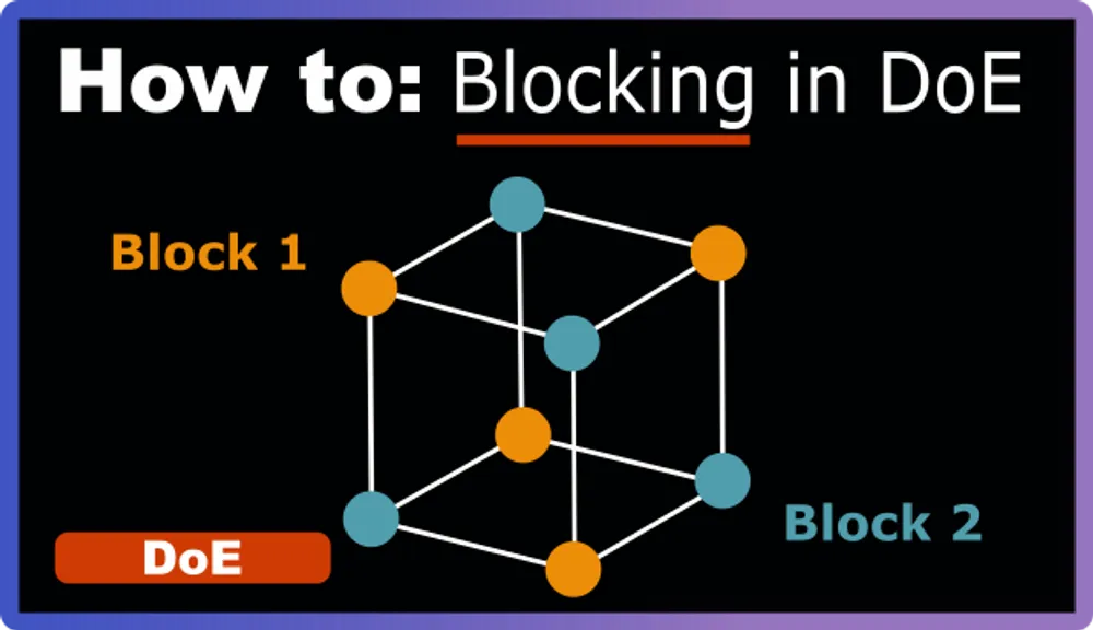
When you can’t fit all your experimental runs into a single block (same batch, same day, same conditions), you need to split them across multiple blocks. But here’s the catch: you can’t just randomly split them. You need to be strategic about it.

This is where confounding comes in. You deliberately confound a factor or interaction with your blocking variable. In practical terms, this means you sacrifice your ability to estimate one effect (usually a high-order interaction you don’t care about) in order to create balanced blocks.

The key assumption is that the blocking factor has an additive effect. It shifts all responses up or down by the same amount, without interacting with your experimental factors.

For a 2⁴ factorial design with two blocks, you typically confound the four-way interaction (T×P×CoF×RPM) with blocks. This gives you two balanced blocks of 8 runs each, while preserving all main effects and two-way interactions.

A Practical Example

Let’s use our familiar filtration rate example, a 2⁴ factorial design testing four factors:

• T – Temperature (20°C vs. 40°C)
• P – Pressure (1 bar vs. 3 bar)
• CoF – Concentration of Formaldehyde (2% vs. 6%)
• RPM – Agitation speed (100 vs. 300)

Response: Filtration rate (arbitrary units)

Here’s our complete dataset (16 runs) with coded levels:

Run	T	P	CoF	RPM	Filtration Rate
1	-1	-1	-1	-1	45
2	+1	-1	-1	-1	71
3	-1	+1	-1	-1	48
4	+1	+1	-1	-1	65
5	-1	-1	+1	-1	68
6	+1	-1	+1	-1	60
7	-1	+1	+1	-1	80
8	+1	+1	+1	-1	65
9	-1	-1	-1	+1	43
10	+1	-1	-1	+1	100
11	-1	+1	-1	+1	45
12	+1	+1	-1	+1	104
13	-1	-1	+1	+1	75
14	+1	-1	+1	+1	86
15	-1	+1	+1	+1	70
16	+1	+1	+1	+1	96

When we analyze this data, we get the following main effects:

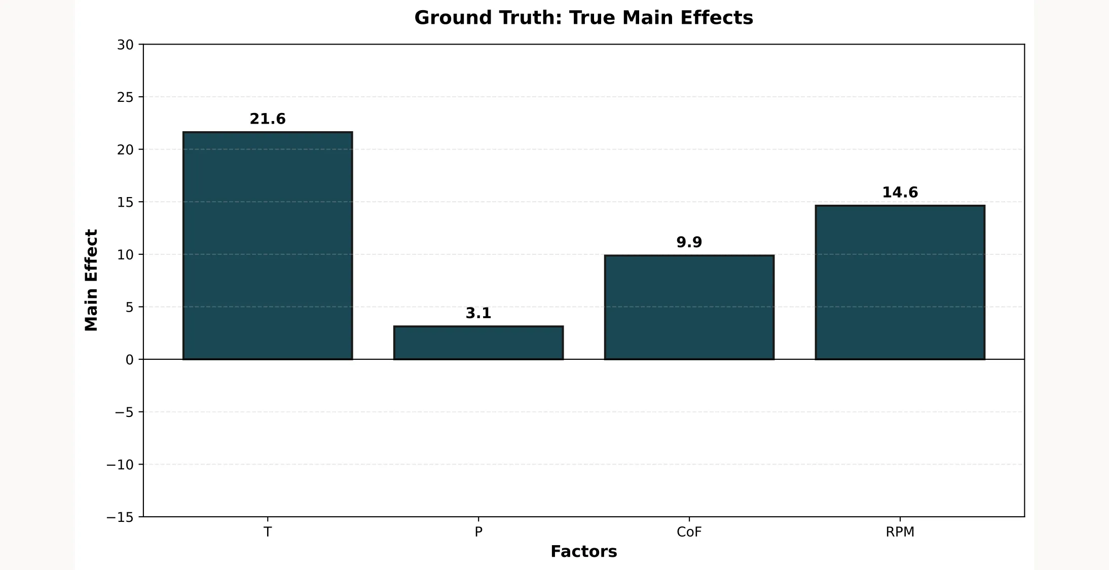
These are our ground truth values. Now let’s see what happens when a systematic error enters the picture and why planning your blocking strategy matters.

Scenario 1: Without Blocking

Imagine you run this experiment over two days without thinking about blocking. You simply run experiments in standard order: runs 1-8 on Day 1, runs 9-16 on Day 2. Unknown to you, there is some unknown variable on Day 1 that adds +20 filtration rate to all your measurements.

Here’s the problem: in standard order, all runs with RPM = -1 happen on Day 1, and all runs with RPM = +1 happen on Day 2.

Run	T	P	CoF	RPM	Day	True	With Error
1	-1	-1	-1	-1	1	45	65
2	+1	-1	-1	-1	1	71	91
3	-1	+1	-1	-1	1	48	68
4	+1	+1	-1	-1	1	65	85
5	-1	-1	+1	-1	1	68	88
6	+1	-1	+1	-1	1	60	80
7	-1	+1	+1	-1	1	80	100
8	+1	+1	+1	-1	1	65	85
9	-1	-1	-1	+1	2	43	43
10	+1	-1	-1	+1	2	100	100
11	-1	+1	-1	+1	2	45	45
12	+1	+1	-1	+1	2	104	104
13	-1	-1	+1	+1	2	75	75
14	+1	-1	+1 oz	+1	2	86	86
15	-1	+1	+1	+1	2	70	70
16	+1	+1	+1	+1	2	96	96

When you analyze this data, the RPM effect is completely wrong:

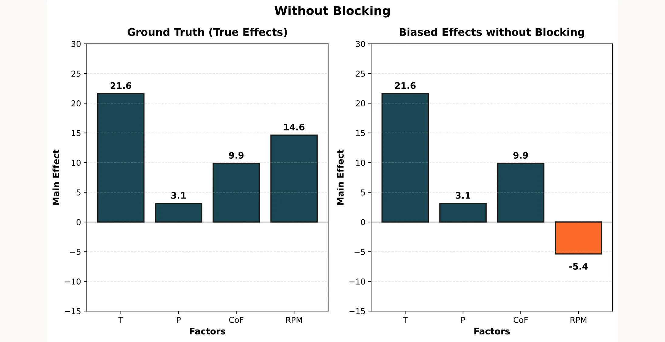
• True RPM effect: +14.6
• Measured RPM effect: -5.4
• Bias: -20.0 units!

The other factors (T, P, CoF) are fine because they’re balanced across both days. But RPM? Completely compromised. You’d conclude that higher RPM decreases filtration rate when actually it increases it.

This is what happens when you don’t plan for blocking.

Scenario 2: With Blocking

Now let’s say you anticipated running the experiment over two days and planned your design accordingly. Instead of running the experiments sequentially, you create a blocked design by confounding the Block variable with the four-way interaction T×P×CoF×RPM.

Why confound with the four-way interaction? Because:

1. You almost never care about four-way interactions (they’re rarely significant)
2. This keeps all main effects and two-way interactions estimable
3. You get two perfectly balanced blocks of 8 runs each

Here’s how you assign runs to blocks using the four-way interaction. First, multiply each column to create the effect of the four-way interaction. Then you assign every +1 to block 1 and every -1 to block 2.

Run	T	P	CoF	RPM	T×P×CoF×RPM	Block
1	-1	-1	-1	-1	+1	1
2	+1	-1	-1	-1	-1	2
3	-1	+1	-1	-1	-1	2
4	+1	+1	-1	-1	+1	1
5	-1	-1	+1	-1	-1	2
6	+1	-1	+1	-1	+1	1
7	-1	+1	+1	-1	+1	1
8	+1	+1	+1	-1	-1	2
9	-1	-1	-1	+1	-1	2
10	+1	-1	-1	+1	+1	1
11	-1	+1	-1	+1	+1	1
12	+1	+1	-1	+1	-1	2
13	-1	-1	+1	+1	+1	1
14	+1	-1	+1	+1	-1	2
15	-1	+1	+1	+1	-1	2
16	+1	+1	+1	+1	+1	1

Notice how Block 1 contains runs 1, 4, 6, 7, 10, 11, 13, 16 and Block 2 contains runs 2, 3, 5, 8, 9, 12, 14, 15. Each block has exactly 4 runs at the low level and 4 runs at the high level for every factor. Perfect balance!

Introducing the Systematic Error

Now the same thing happens: on Day 1 (Block 1) something happens that adds +20 to all measurements. Here’s the data:

Run	T	P	CoF	RPM	Block	True	With Error
1	-1	-1	-1	-1	1	45	65
2	+1	-1	-1	-1	2	71	71
3	-1	+1	-1	-1	2	48	48
4	+1	+1	-1	-1	1	65	85
5	-1	-1	+1	-1	2	68	68
6	+1	-1	+1	-1	1	60	80
7	-1	+1	+1	-1	1	80	100
8	+1	+1	+1	-1	2	65	65
9	-1	-1	-1	+1	2	43	43
10	+1	-1	-1	+1	1	100	120
11	-1	+1	-1	+1	1	45	65
12	+1	+1	-1	+1	2	104	104
13	-1	-1	+1	+1	1	75	95
14	+1	-1	+1	+1	2	86	86
15	-1	+1	+1	+1	2	70	70
16	+1	+1	+1	+1	1	96	116

Calculating Main Effects

Here’s the beautiful result: because Block is confounded with the four-way interaction, even with the +20 systematic error on Block 1, the actual effects you calculate are not compromised:

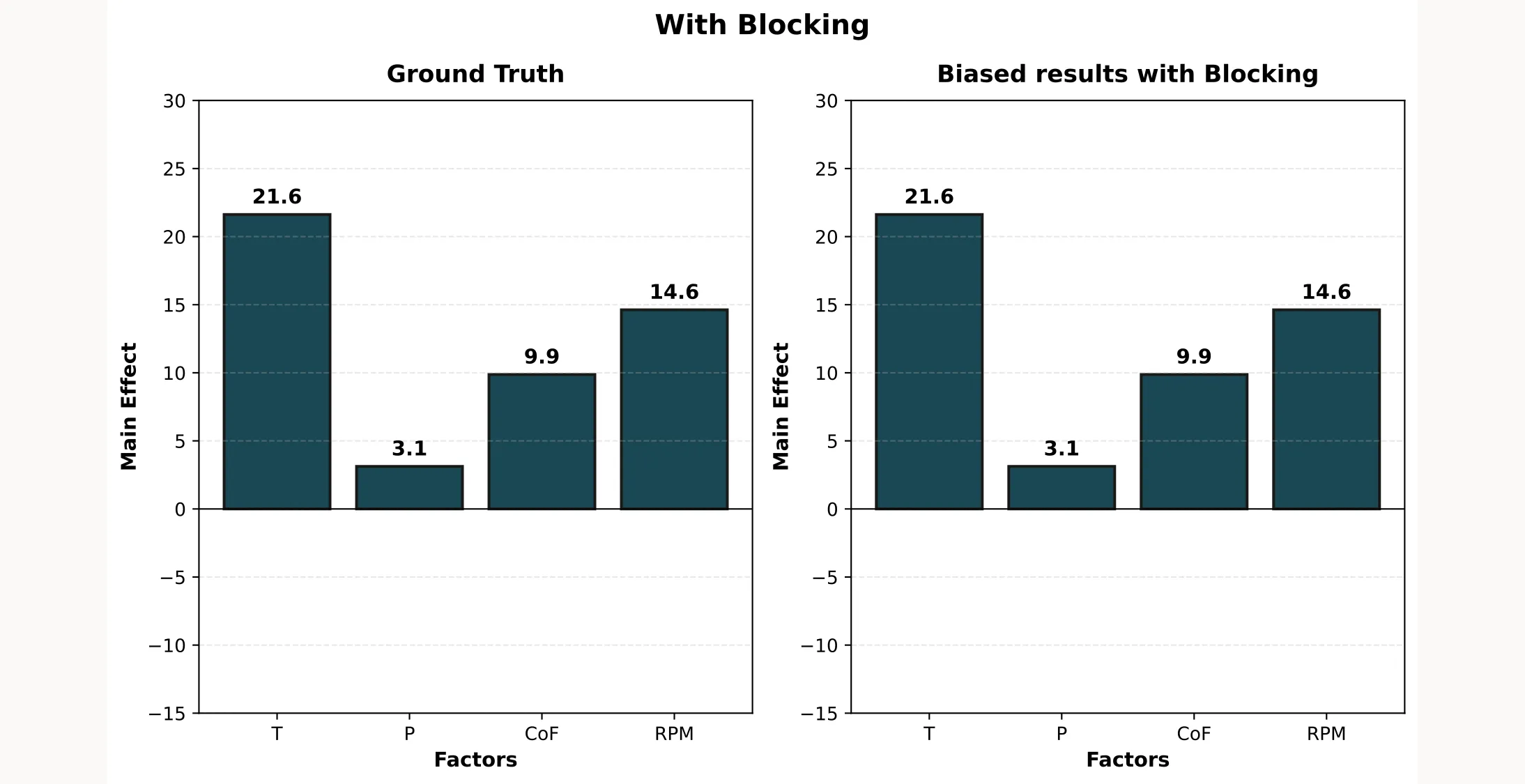
Because each block has exactly 4 runs at the low level and 4 runs at the high level for every factor. When the +20 error hits Block 1, it affects 4 low and 4 high runs for T, P, CoF, and RPM equally. The bias cancels out when calculating main effects!

Compare this to Figure 2 above, where RPM was completely confounded with Day. There, all 8 low-RPM runs got the error, completely biasing the RPM estimate.

You even get:

1. An estimate of the block effect (+20 in this case)
2. A warning that something varied between days and you can investigate the issue
3. Cleaner error variance because the block effect is explained, not treated as noise

And all that without any additional effort. You only had to think about it upfront.

But What About Randomization?

You might be thinking: “Can’t I just randomize the run order? Won’t that solve the problem?”

Let’s see. If you had randomized the run order, the +20 error would hit 8 random runs instead of the first 8:

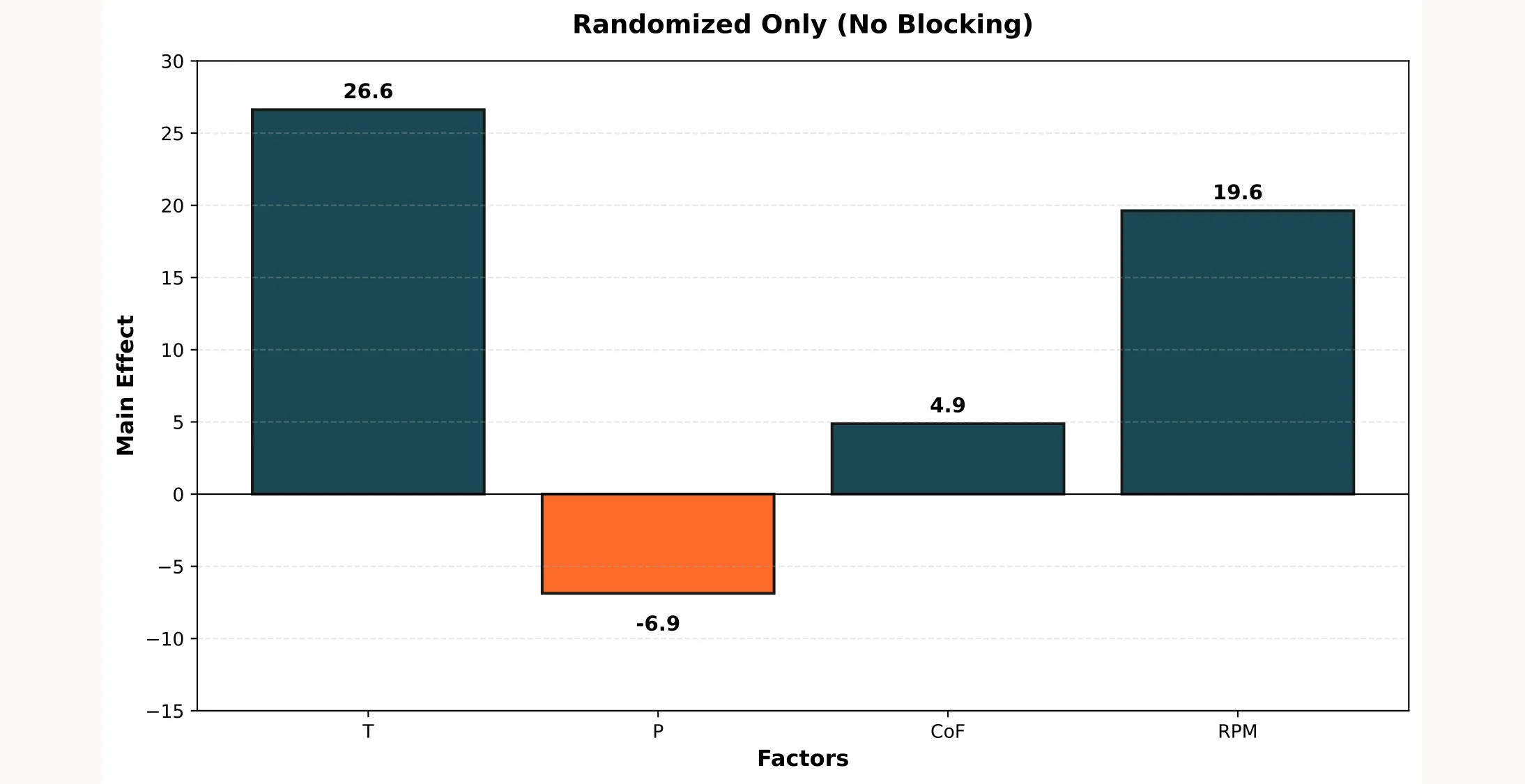
With randomization alone:

• The bias doesn’t concentrate on one factor (good!)
• But all effects become noisier (bad!)
• You still don’t remove the systematic error (bad!)

Here’s the key distinction:

Randomization protects against unknown sources of bias. It prevents correlations between uncontrolled variables and your factors.

Blocking handles known sources of variability. It actively removes their effect from your analysis.

You need both. Randomize within blocks to protect against unknown confounders. Block to control for known nuisance variables.

A Reference Table to Find the Right Blocking Strategy

So far we’ve seen blocking with 2 blocks for a 2⁴ design. But what if you need more blocks? Or have a different number of factors?

As you increase the number of blocks, you sacrifice design resolution. More interactions become confounded with block effects. The table below (adapted from Montgomery’s Design and Analysis of Experiments) shows suggested blocking arrangements for 2^k factorial designs:

Factors (k)	Blocks	Block Size	Effects to Generate Blocks	Interactions Confounded with Blocks
3	2	4	ABC	ABC
	4	2	AB, AC	AB, AC, BC
4	2	8	ABCD	ABCD
	4	4	ABC, ACD	ABC, ACD, BD
	8	2	AB, BC, CD	AB, BC, CD, AC, BD, AD, ABCD
5	2	16	ABCDE	ABCDE
	4	8	ABC, CDE	ABC, CDE, ABDE
	8	4	ABE, BCE, CDE	ABE, BCE, CDE, AC, ABCD, BD, ADE
	16	2	AB, AC, CD, DE	All 2- and 4-factor interactions
6	2	32	ABCDEF	ABCDEF
	4	16	ABCF, CDEF	ABCF, CDEF, ABDE
	8	8	ABEF, ABCD, ACE	ABEF, ABCD, ACE, BCF, BDE, CDEF, ADF
7	2	64	ABCDEFG	ABCDEFG
	4	32	ABCFG, CDEFG	ABCFG, CDEFG, ABDE

How to read this table:

• Factors (k): Number of factors in your design
• Blocks: Number of blocks you want (must be a power of 2)
• Block Size: Number of runs per block (2^k / number of blocks)
• Effects to Generate Blocks: The interactions you use to assign runs to blocks
• Interactions Confounded: What you lose the ability to estimate independently

Key insight: With 2 blocks, you only lose the highest-order interaction. With more blocks, you start losing lower-order interactions too. Choose the smallest number of blocks that fits your practical constraints.

For our 2⁴ filtration rate example, we used 2 blocks of 8 runs each, confounding ABCD (the four-way interaction), exactly what the table recommends.

Try It Yourself

I’ve created an interactive Jupyter notebook that walks through all the examples in this post with Python code you can modify and run yourself. You can download it here.

Up next:

<< Why Blocking Matters (Real Example) >>

<< Principles of DoE: Randomization, Replication, Blocking >>