Understanding the ANOVA Table Output
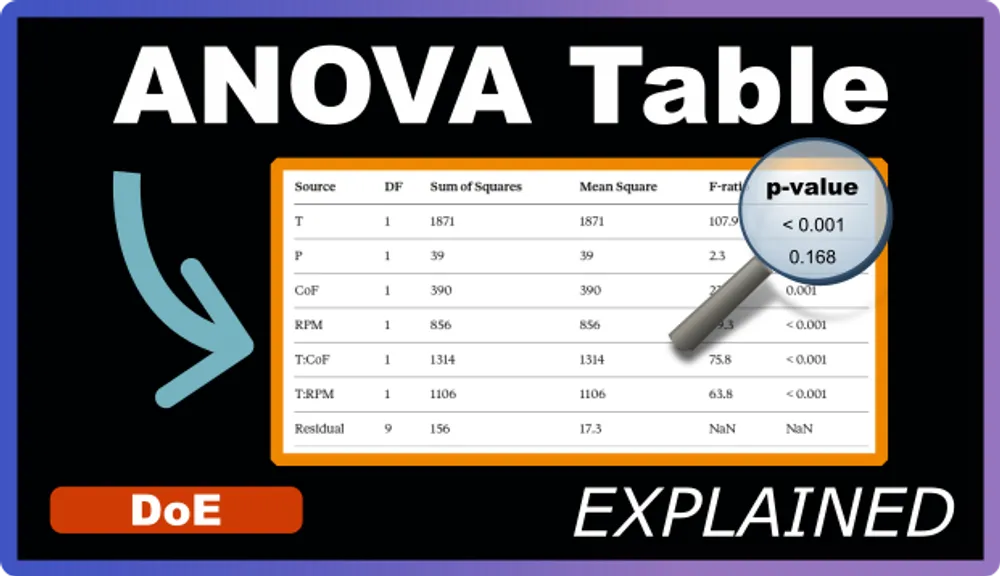
In our previous post, we learned how to perform ANOVA to build statistically justified models. We ran the analysis and got this table:
| Source | DF | Sum of Squares | Mean Square | F-ratio | p-value |
|---|---|---|---|---|---|
| T | 1 | 1871 | 1871 | 107.9 | < 0.001 |
| P | 1 | 39 | 39 | 2.3 | 0.168 |
| CoF | 1 | 390 | 390 | 22.5 | 0.001 |
| RPM | 1 | 856 | 856 | 49.3 | < 0.001 |
| T:CoF | 1 | 1314 | 1314 | 75.8 | < 0.001 |
| T:RPM | 1 | 1106 | 1106 | 63.8 | < 0.001 |
| Residual | 9 | 156 | 17.3 | NaN | NaN |
But what does all this actually mean? Let’s decode it column by column.
The Source Column: What Are We Testing?
The Source column lists every parameter in your model. Each row represents one piece of your model equation that ANOVA is evaluating.
In our filtration rate example:
- T, P, CoF, RPM are the main effects (the individual factors)
- T:CoF and T:RPM are interaction terms (how factors work together)
- Residual is special—it represents everything your model doesn’t explain, the leftover variation
Think of Source as the defendants in a trial. Each one is being judged on whether it contributes meaningfully to explaining your results.
Degrees of Freedom (DF): How Much Independent Information?
Degrees of freedom tells you how many independent pieces of information are used to calculate each statistic. For most single terms in a factorial design, DF equals 1 because you’re comparing two levels (low and high).
Here’s the intuition: when you test Temperature, you’re really asking, “Is the average response at high temperature different from the average at low temperature?” That’s one independent comparison, so DF = 1.
The Residual DF (9 in our example) depends on your total number of runs minus the number of parameters you’re estimating. We have 16 runs, estimate 6 parameters plus an intercept (7 total), leaving us with 16 − 7 = 9 degrees of freedom for error. These 9 independent pieces of leftover information help us estimate how noisy our data is.
Sum of Squares (SS): Total Variation Attributed
Sum of Squares measures the total amount of variation in your response that can be attributed to each source. Think of it as the total distance your predictions move when you include that parameter.
Looking at our table:
- T has SS = 1871: Temperature causes a lot of variation in filtration rate
- P has SS = 39: Pressure causes very little variation
- T:CoF has SS = 1314: The Temperature-Formaldehyde interaction causes substantial variation
The larger the Sum of Squares, the more that parameter is “moving” your response values around. But raw SS values are hard to compare directly because they depend on how many measurements you have. That’s where Mean Square comes in.
Mean Square (MS): Average Variation
Mean Square is simply Sum of Squares divided by Degrees of Freedom. It’s the average amount of variation per independent piece of information.
Mean Square = Sum of Squares ÷ DF
For most terms in our table, DF = 1, so MS equals SS. But this becomes important when comparing different sources with different degrees of freedom, or when looking at the Residual.
The Residual Mean Square (17.3 in our example) is particularly important. It represents the average amount of random noise in your data—the baseline variation you’d expect from measurement error and other uncontrolled factors. This becomes our benchmark for what “normal variation” looks like.
F-ratio: Signal Compared to Noise
The F-ratio is where ANOVA makes its key comparison. It divides the Mean Square of each parameter by the Residual Mean Square:
F-ratio = Mean Square (parameter) ÷ Mean Square (residual)
Think of it as a signal-to-noise ratio. The F-ratio asks: “How much bigger is the effect of this parameter compared to random noise?”
Let’s look at two examples from our table:
Temperature (T): F-ratio = 107.9 This means the variation caused by Temperature is 107.9 times larger than the baseline noise. That’s a huge signal.
Pressure (P): F-ratio = 2.3 Pressure’s effect is only 2.3 times larger than noise. That’s a weak signal that could easily be confused with random variation.
A rule of thumb: F-ratios much larger than 5 typically indicate real effects. F-ratios near 1 suggest the parameter isn’t doing much more than noise.
p-value: Is It Real or Just Luck?
The p-value answers a simple question: “If this parameter truly had no effect, what’s the probability I’d see an F-ratio this large just by random chance?”
Here’s how to read it:
p < 0.001 (like Temperature): There’s less than a 0.1% chance you’d see this result if Temperature didn’t matter. It’s almost certainly a real effect.
p = 0.168 (like Pressure): There’s a 16.8% chance you’d see this result even if Pressure had no effect. That’s not convincing evidence.
The standard threshold is p < 0.05, meaning we accept a 5% risk of being wrong. Parameters below this threshold are considered statistically significant.
In our table, T, CoF, RPM, T:CoF, and T:RPM all have p-values well below 0.05. Only Pressure fails the test with p = 0.168.
Important reminder: A significant p-value means the effect is real, but it doesn’t tell you if the effect is large enough to care about. Always consider both statistical significance and practical importance.
The Residual Row: What’s Left Over
The Residual row is unique—it doesn’t represent a parameter you tested. Instead, it captures all the variation in your data that your model can’t explain.
Think of your total variation as a pizza. Each parameter’s Sum of Squares is a slice that parameter claims. The Residual is whatever slices are left after all parameters take their share. It includes measurement error, experimental noise, and effects of factors you didn’t measure.
The Residual Mean Square (17.3) sets the scale for what “normal variation” looks like in your experiment. This is the number that every other parameter is compared against via the F-ratio.
A good model has a relatively small Residual Sum of Squares compared to the parameter Sum of Squares. If your Residual is huge, it means your model isn’t explaining much.
Reading the Table as a Whole
Now let’s put it all together. When you look at an ANOVA table, scan it like this:
- Check the p-values first: Which parameters are below 0.05? Those are your keepers.
- Look at the F-ratios: How strong are the significant effects? Larger F-ratios mean more confident conclusions.
- Compare the Sum of Squares: Which parameters are driving the most variation? These are your most impactful factors.
- Consider the Residual: Is it reasonably small compared to your parameter effects?
In our filtration rate example, the story is clear: Temperature, Formaldehyde concentration, and RPM all matter. Two interactions (T:CoF and T:RPM) are also important. Pressure doesn’t make the cut—its small F-ratio and high p-value suggest it’s not contributing beyond noise.
Key Takeaways
The ANOVA table is your statistical report card for every parameter in your model. Each column tells part of the story: Sum of Squares shows how much variation a parameter captures, the F-ratio compares that to baseline noise, and the p-value tells you whether to believe it’s real.
When building models, the p-value is your main decision tool. Keep parameters below your significance threshold (typically 0.05) and remove those above it. But don’t forget to look at the practical importance too—a statistically significant effect might still be too small to matter in your real process.