When you’re trying to optimize a process, you typically start with a design that gives you a linear model, like a fractional or full factorial design. But most of the time, you’re not in the region of optimal performance yet and you need a systematic way to climb toward better performance from your starting point. The path of steepest ascent is a core technique in response surface methodology (RSM) that helps you reach your optimum as efficiently as possible.

What Is the Path of Steepest Ascent?

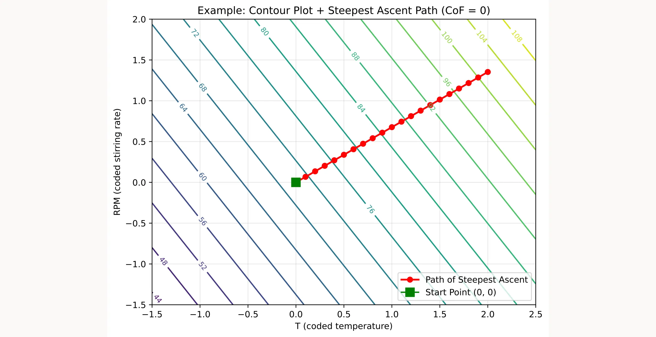
The path of steepest ascent represents the direction of maximum increase in your response. On a contour plot, this path runs perpendicular to the contour lines, giving you the most direct route uphill toward better performance.

It applies specifically to linear models. Once you’ve moved into a region where curvature becomes important and you’ve fitted a quadratic model, you’ll switch to ridge analysis instead. Ridge analysis is something we cover in a future article.

The calculation is relatively straightforward, though the approach differs slightly depending on whether you have interactions between factors. If you want to follow along with code, here’s a Python example.

Modelling the Path of Steepest Ascent

Without Interaction Terms

1. Fit a First-Order Model
   Use experimental data (in coded units) to fit a first-order linear regression model:

   $$\hat{y} = b_0 + b_1 x_1 + b_2 x_2 + \dots + b_m x_m$$

2. Extract Coefficients
   The estimated coefficients $(b_1, b_2, \dots, b_m)$ define the gradient direction of ascent.
   The magnitude of each coefficient determines the relative step size, and its sign indicates the direction for maximization.

3. Choose a Reference Variable and Step Size $(\Delta x_j)$
   Select one variable $j$ as the reference and assign it a small step size $(\Delta x_j)$ in coded units.

4. Calculate Relative Steps for Other Variables $(\Delta x_k)$
   Compute relative steps for the remaining variables so that movement follows the gradient:

   $$\Delta x_k = \frac{b_k}{b_j}\,\Delta x_j$$

5. Example
   For the first-order model:

   $$FR = 70.0625 + 10.8125\,T + 7.3125\,RPM + 4.9375\,CoF$$

   Using temperature as the reference variable with $\Delta T = 0.1$:

   $$\Delta RPM = \frac{b_{RPM}}{b_T}\,\Delta T = \frac{7.3125}{10.8125}\times 0.1 = 0.0676$$ $$\Delta CoF = \frac{b_{CoF}}{b_T}\,\Delta T = \frac{4.9375}{10.8125}\times 0.1 = 0.0457$$

→ This means that when temperature increases by 0.1 (coded units), RPM should increase by 0.0676 and CoF by 0.0457 to move along the path of steepest ascent.

With 2FI Interaction Terms

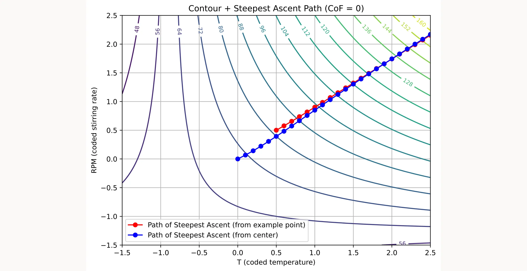
When interaction terms are present, the direction of steepest ascent is no longer constant. It depends on where you are in the design space. Each factor’s slope changes with the levels of the others.

1. Fit a Linear Model with Interactions (2FI)
   Extend the first-order model to include two-factor interactions:

   $$\hat{y} = b_0 + \sum b_i x_i + \sum_{i<j} b_{ij} x_i x_j$$

2. Compute Local Slopes at the Current Settings $x_c$
   With interactions, each slope depends on the current levels of the other variables.
   For each variable $k$:

   $$s_k = b_k + \sum_{i \neq k} b_{ki}\, x_{c,i}$$

   At the design center ($x_c = 0$), $s_k = b_k$, so the direction equals the simple first-order case.

3. Pick a Reference Variable and Small Step $(\Delta x_j)$
   Choose one variable $j$ as the reference and define a small step $\Delta x_j$ in coded units.
   Then calculate the relative steps using the ratios of local slopes:

   $$\Delta x_k = \frac{s_k}{s_j}\,\Delta x_j \quad (k \neq j)$$

   If there are no interactions, $s_k = b_k$, and this simplifies to the non-interacting case.

4. Iterate and Recalculate as You Move
   Because interactions can curve the response surface, the ascent direction may shift as you move. After each step, recompute the local slopes $s_k$.
   When improvements taper off, fit a second-order model and apply ridge analysis to locate the optimum.

5. Example

   Term	Coefficient
   Intercept	70.0625
   T	10.8125
   RPM	7.3125
   CoF	4.9375
   T:RPM	8.3125
   T:CoF	-9.0625

   Suppose you are at $x_T = 0.5$, $x_{RPM} = 0.5$, and $x_{CoF} = 0$.
   Compute the local slopes:

   $$s_T = b_T + b_{T,RPM}\,x_{RPM} + b_{T,CoF}\,x_{CoF} = 10.8125 + 8.3125(0.5) - 9.0625(0) = 14.9688$$ $$s_{RPM} = b_{RPM} + b_{T,RPM}\,x_T = 7.3125 + 8.3125(0.5) = 11.4688$$ $$s_{CoF} = b_{CoF} + b_{T,CoF}\,x_T = 4.9375 - 9.0625(0.5) = 0.4063$$

   Using $T$ as the reference variable with $\Delta T = 0.1$:

   $$\Delta RPM = \frac{s_{RPM}}{s_T}\,\Delta T = \frac{11.4688}{14.9688}\times 0.1 = 0.0766$$ $$\Delta CoF = \frac{s_{CoF}}{s_T}\,\Delta T = \frac{0.4063}{14.9688}\times 0.1 = 0.0027$$

→ When increasing $T$ by 0.1, increase $RPM$ by 0.0766 and $CoF$ by only 0.0027.
→ After each step, re-evaluate $s_k$ to account for curvature introduced by the interactions.

In Practice…

…you would now move along the path of steepest ascent and pick a step size for verification experiments to confirm you’re still on track and your response is still improving. You can stop once you reach a certain threshold you’re happy with. Or, once improvements become marginal, you can run another design to fit a second-order model, like a Central Composite design or a Box-Behnken design.

Summary

The path of steepest ascent gives you a systematic way to move toward better performance:

1. Fit a first-order model from your screening or first-stage experiments
2. Extract the coefficients to understand the gradient direction
3. Choose a reference variable and a practical step size
4. Calculate proportional steps for other variables based on their coefficients
5. For models with interactions, compute local slopes at each position and recalculate as you move
6. Take small steps, measure actual responses, and iterate
7. Stop when improvements level off, then consider fitting a quadratic model

Up next

<< Introducing Fractional & Central Composite Designs >>

<< Create a Box-Behnken Design in Python >>

<< Create a Central Composite Design in Python >>