If your full or fractional factorial pointed you in the right direction but you still can’t answer “where is the optimum?”, it’s time for a Central Composite Design (CCD). In this post, I’ll build directly on the ideas from Introducing Fractional & Central Composite Designs and walk through a practical, step‑by‑step CCD using the same filtration example from A step by step example of a full factorial design. We’ll keep it hands‑on, focus on what matters in practice, and compare effort versus insight along the way.

When to use a CCD (recap)

A CCD is the right tool when:

• You’ve already screened and narrowed to a few important factors.
• You suspect curvature or need to locate a maximum/minimum.
• You want a predictive model you can trust near the optimum.

In short: don’t start with a CCD. Use it after screening (fractional or full factorial) when you’re ready to fine‑tune.

CCDs and Response Surface Methodology (RSM)

Central composite designs are a core piece of Response Surface Methodology—a family of designs and analyses used to model curved (quadratic) relationships and search for optima. RSM typically uses:

• Central Composite Designs (this post)
• Box–Behnken Designs

The goal is a quadratic model that is accurate in the region of interest so you can navigate to the best settings confidently.

CCD vs. 3‑level full factorial: run counts

Before diving into the example, let’s address the obvious alternative. You could explore curvature using a 3-level full factorial design, testing each factor at low, middle, and high levels. While this works, it’s expensive. A CCD is much more efficient.

Example with 4 factors (k = 4):

• 3‑level full factorial: 3^4 = 81 runs
• CCD (rotatable): 2^4 factorial points (16) + 2k axial/star points (8) + center replicates (e.g., 5) ≈ 29 runs

Even with extra center points for pure error, a CCD achieves basically the same modeling capability with less than one‑third the runs required by a 3‑level full factorial design.

Filtration rate example

Let’s return to our filtration process from our full factorial example.

• T — Temperature: 20–40°C
• P — Pressure: 1–3 bar
• CoF — Formaldehyde concentration: 2–6%
• RPM — Agitation speed: 100–300

We again work in coded units to keep the math clean and comparable across factors.

Note: In the full factorial design we already established that pressure is an insignificant parameter. We could drop it from our analysis and skip including it in our central composite design, saving 2 experimental runs by eliminating 2 star points (for pressure). Since the experimental effort is negligible, we’ll leave it in and use it to estimate error.

CCD design

A central composite design combines three types of experimental points:

1. Factorial points: The corners of our design space (coded as ±1)
2. Center points: Multiple runs at the center of the design space (coded as 0)
3. Star points: Extended points beyond the factorial range (coded as ±α)

For our example, this translates to:

Factor	Low (−1)	Center (0)	High (+1)
T	20	30	40
P	1	2	3
CoF	2	4	6
RPM	100	200	300

Choosing the star point distance (alpha)

The star point distance α determines how far beyond your original factorial range you’ll test. Common choices are:

• Rotatable design with α = 2^(k/4): You obtain a rotatable design. This gives uniform prediction precision at equal distance from the center in any direction.
• Face-centered design with α = 1: If ±α exceeds safe/feasible real‑unit limits, use a face‑centered CCD (α = 1). It’s less rotatable but often more practical with hard constraints.

In our example we use a face-centered design as using a rotatable design would require to test P, CoF and RPM for -alpha at 0 which is practically not feasible. This is how the design table looks like. We added 5 center points to estimate error:

Run	Point Type	T	P	CoF	RPM	Filtration Rate
1	Factorial	−1	−1	−1	−1	45.0
2	Factorial	+1	−1	−1	−1	71.0
3	Factorial	−1	+1	−1	−1	48.0
4	Factorial	+1	+1	−1	−1	65.0
5	Factorial	−1	−1	+1	−1	68.0
6	Factorial	+1	−1	+1	−1	60.0
7	Factorial	−1	+1	+1	−1	80.0
8	Factorial	+1	+1	+1	−1	65.0
9	Factorial	−1	−1	−1	+1	43.0
10	Factorial	+1	−1	−1	+1	100.0
11	Factorial	−1	+1	−1	+1	45.0
12	Factorial	+1	+1	−1	+1	104.0
13	Factorial	−1	−1	+1	+1	75.0
14	Factorial	+1	−1	+1	+1	86.0
15	Factorial	−1	+1	+1	+1	70.0
16	Factorial	+1	+1	+1	+1	96.0
17	Star	+1	0	0	0	67.3
18	Star	−1	0	0	0	45.1
19	Star	0	+1	0	0	70.1
20	Star	0	−1	0	0	67.7
21	Star	0	0	+1	0	73.3
22	Star	0	0	−1	0	63.4
23	Star	0	0	0	+1	76.6
24	Star	0	0	0	−1	61.4
25	Center	0	0	0	0	69.7
26	Center	0	0	0	0	70.5
27	Center	0	0	0	0	69.7
28	Center	0	0	0	0	69.7
29	Center	0	0	0	0	70.3

Note: The factorial points are the same combinations we tested in our original 2-level factorial example, but now we’re adding star points and center points to capture curve relationships. You do not need to repeat the full factorial points but can use the results from the full factorial experiment.

Modeling the response surface

Unlike our previous linear analysis (see here), CCD allows us to fit a quadratic model that can capture curvature. The general process remains the same as with the linear model—we build it through backward elimination or forward selection (check here if you need a refresher)—but this time we also include quadratic model terms.

We can start with the linear model from our full factorial design:

Filtration Rate = β₀ + β₁·T + β₂·CoF + β₃·RPM + β₁₂·(T×CoF) + β₁₃·(T×RPM)

Then extend it to include quadratic terms for the main effects:

Filtration Rate = β₀ + β₁·T + β₂·CoF + β₃·RPM + β₁₂·(T×CoF) + β₁₃·(T×RPM) + β₁₁·T² + β₂₂·CoF² + β₃₃·RPM²

The resulting ANOVA table shows:

Source	DF	Sum of Squares	Mean Square	F-ratio	p-value
Intercept	1	43624.25	43624.25	2745.30	< 0.001
T	1	2115.32	2115.32	133.12	< 0.001
CoF	1	438.77	438.77	27.61	< 0.001
RPM	1	972.11	972.11	61.18	< 0.001
T×CoF	1	1314.06	1314.06	82.69	< 0.001
T×RPM	1	1105.56	1105.56	69.57	< 0.001
RPM²	1	75.19	75.19	4.73	0.042
T²	1	165.06	165.06	10.39	0.004
CoF²	1	58.06	58.06	3.65	0.070
Residual	20	317.81	15.89	-	-

The CoF² term has a p-value of 0.070, which exceeds our significance criterion of p < 0.05, making it non-significant. We’ll remove it to keep only the significant terms:

Source	DF	Sum of Squares	Mean Square	F-ratio	p-value
Intercept	1	46014.09	46014.09	2570.80	< 0.001
T	1	2115.32	2115.32	118.18	< 0.001
CoF	1	438.77	438.77	24.51	< 0.001
RPM	1	972.11	972.11	54.31	< 0.001
T×CoF	1	1314.06	1314.06	73.42	< 0.001
T×RPM	1	1105.56	1105.56	61.77	< 0.001
RPM²	1	168.85	168.85	9.43	0.006
T²	1	113.37	113.37	6.33	0.020
Residual	21	375.87	17.90	-	-

Visualize the response surface

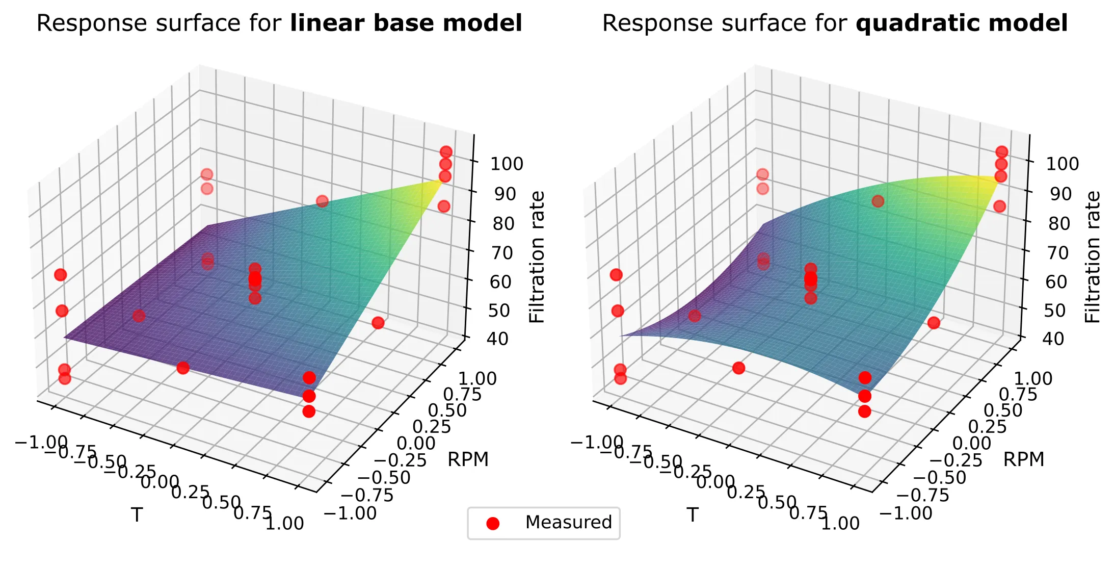
Several visualization methods can help us understand the response surface. A 3D surface plot is one option:

The response surface for the quadratic model shows subtle curvature compared to the strictly linear base model. This curvature appears to capture how filtration rate changes with different factors slightly better than a purely linear relationship.

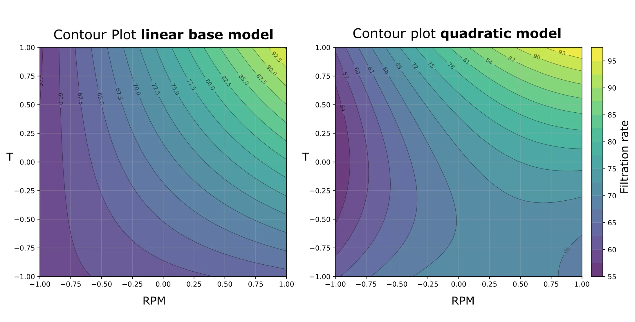
Another way to visualize the response surface is through contour plots. They show “equal response” lines, much like elevation contours on a topographic map. The drawback is that you cannot directly display your measured values within the plot to get an idea of how good the fit is. But it is anyway better to rely on residual analysis for model evaluation.

Comparing the linear vs. quadratic model performance

In this example, the quadratic model provides only a modest improvement over the linear model, as we can see when directly comparing measured and predicted values for both approaches. The quadratic model is slightly better at predicting the response, but the improvement is relatively small. This tells us that our original linear model from the factorial design was already capturing most of the important relationships in this system.

Run	T	P	CoF	RPM	Actual Rate	Data Source	Linear Pred	Quadratic Pred	Linear Error	Quadratic Error
1	−1	−1	−1	−1	45.0	Full Factorial	44.9	45.4	−0.1	0.4
2	+1	−1	−1	−1	71.0	Full Factorial	68.1	68.6	−2.9	−2.4
3	−1	+1	−1	−1	48.0	Full Factorial	44.9	45.4	−3.1	−2.6
4	+1	+1	−1	−1	65.0	Full Factorial	68.1	68.6	3.1	3.6
5	−1	−1	+1	−1	68.0	Full Factorial	72.9	73.4	4.9	5.4
6	+1	−1	+1	−1	60.0	Full Factorial	59.9	60.4	−0.1	0.4
7	−1	+1	+1	−1	80.0	Full Factorial	72.9	73.4	−7.1	−6.6
8	+1	+1	+1	−1	65.0	Full Factorial	59.9	60.4	−5.1	−4.6
9	−1	−1	−1	+1	43.0	Full Factorial	43.0	43.5	0.0	0.5
10	+1	−1	−1	+1	100.0	Full Factorial	99.4	99.9	−0.6	−0.1
11	−1	+1	−1	+1	45.0	Full Factorial	43.0	43.5	−2.0	−1.5
12	+1	+1	−1	+1	104.0	Full Factorial	99.4	99.9	−4.6	−4.1
13	−1	−1	+1	+1	75.0	Full Factorial	71.0	71.5	−4.0	−3.5
14	+1	−1	+1	+1	86.0	Full Factorial	91.2	91.7	5.2	5.7
15	−1	+1	+1	+1	70.0	Full Factorial	71.0	71.5	1.0	1.5
16	+1	+1	+1	+1	96.0	Full Factorial	91.2	91.7	−4.8	−4.3
17	+1	0	0	0	67.3	CCD Star	79.7	73.1	12.4	5.8
18	−1	0	0	0	45.1	CCD Star	58.0	51.4	12.9	6.3
19	0	+1	0	0	70.1	CCD Star	68.8	68.0	−1.3	−2.1
20	0	−1	0	0	67.7	CCD Star	68.8	68.0	1.1	0.3
21	0	0	+1	0	73.3	CCD Star	73.8	73.0	0.5	−0.3
22	0	0	−1	0	63.4	CCD Star	63.9	63.1	0.5	−0.3
23	0	0	0	+1	76.6	CCD Star	76.2	82.4	−0.4	5.8
24	0	0	0	−1	61.4	CCD Star	61.5	67.7	0.1	6.3
25	0	0	0	0	69.7	CCD Center	68.8	68.0	−0.9	−1.7
26	0	0	0	0	70.5	CCD Center	68.8	68.0	−1.7	−2.5
27	0	0	0	0	69.7	CCD Center	68.8	68.0	−0.9	−1.7
28	0	0	0	0	69.7	CCD Center	68.8	68.0	−0.9	−1.7
29	0	0	0	0	70.3	CCD Center	68.8	68.0	−1.5	−2.3

Look at the highlighted rows (17-18): these star points demonstrate where the quadratic model actually outperforms the linear model. The linear model struggled to predict these intermediate factor level combinations, while the quadratic model handles them much better. Overall, however, the improvement wasn’t dramatic.

This situation isn’t uncommon. Sometimes quadratic models provide dramatic improvements, especially in optimization problems near a true optimum. Other times, like here, the linear model was already performing well, and the quadratic terms only add incremental value.

The key insight is that we tested for curvature and found it to be minimal in our current operating range. If we had chosen wider factor ranges or were closer to a true optimum, the quadratic effects might have been more pronounced.

What’s next

<< Create a Central Composite Design in Python >>

<< Mathematical models in DoE >>

<< Central composite design vs. Box-Behnken design — coming soon >>