Response Surface Methodology (RSM)
Imagine having a magic button that tells you the perfect combination of temperature, pressure, concentration, and time to maximize your yield. That button doesn’t exist, but Response Surface Methodology (RSM) comes pretty close.
What Response surface methodology is
Response Surface Methodology (RSM) is a collection of statistical and mathematical tools for iterative process optimization. Instead of running one large experiment, RSM improves a process sequentially.
Think of it as a hiking expedition. You can’t see the summit from where you stand, but you can look around, figure out which direction goes uphill, take a few steps, reassess, and repeat. That’s exactly how RSM works.
You start by selecting a small region within your overall experimental space. Don’t try to explore everything at once. Pick a starting point with narrow factor ranges. Run an experiment in that local area, fit a model to understand the response surface, then use that information to decide where to explore next. Each iteration brings you closer to optimal conditions.
Example: Optimizing the yield of a chemical reaction
Let’s say you want to optimize the yield of a chemical reaction with two factors: temperature and reaction time.
Since you have only 2 factors, you can start with a full factorial design, which requires just 4 experiments. Your initial hypothesis is that the optimal conditions lie somewhere within:
- Temperature: 750–850 K
- Reaction time: 2–4 minutes
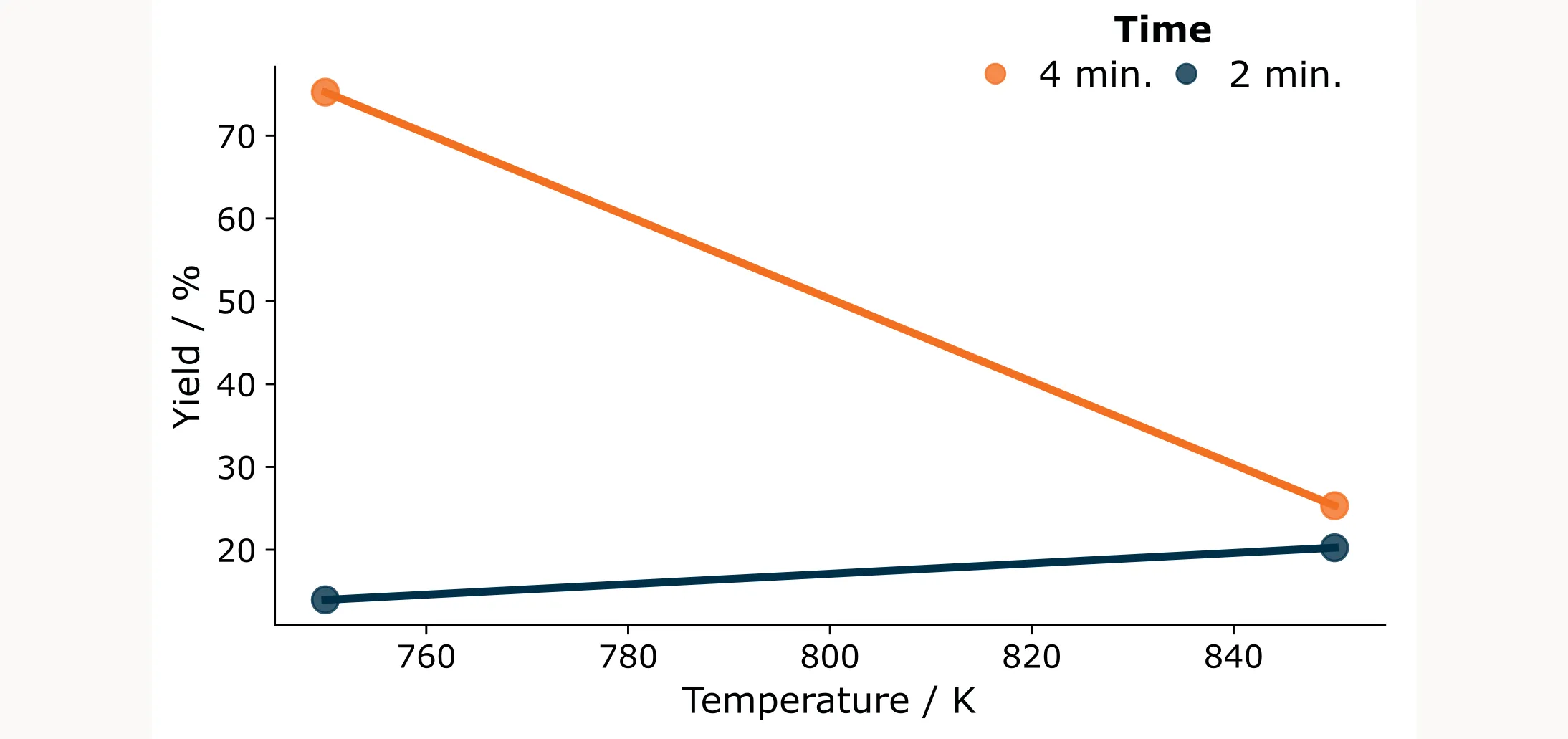
You run the initial full factorial design and obtain the following results:
| Run | Temperature (K) | Time (min) | Yield (%) |
|---|---|---|---|
| 1 | 750 | 2 | 14.0 |
| 2 | 850 | 2 | 20.3 |
| 3 | 750 | 4 | 75.3 |
| 4 | 850 | 4 | 25.3 |
Looking at the results it’s clear that increasing reaction time while decreasing temperature improves the yield. The best result so far is 75.3%, which is decent but leaves room for improvement. The question now is: where should you run your next experiments?
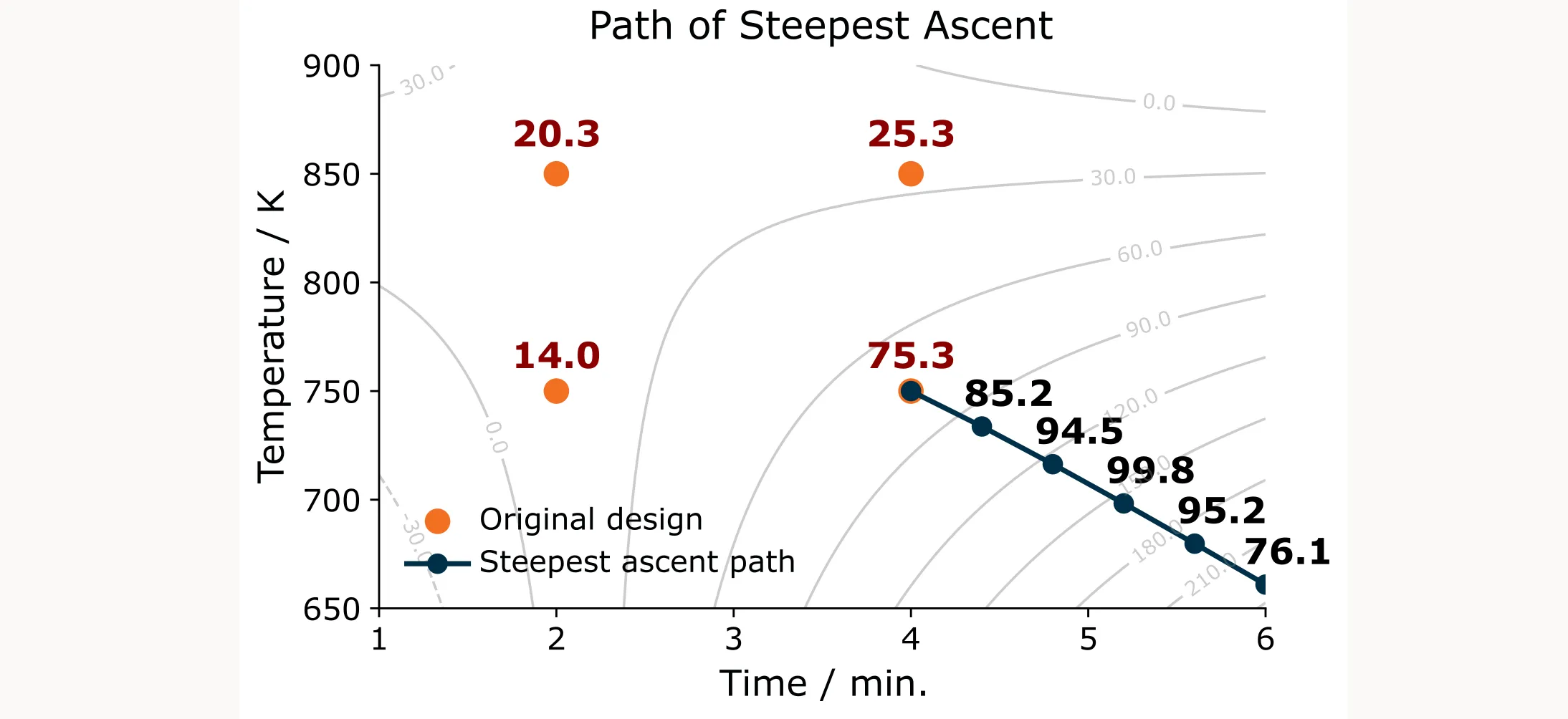
The Path of Steepest Ascent
To improve as quickly as possible, you need to follow the path of steepest ascent, which is the direction that increases your response variable most rapidly.
Here’s how it works: You fit a first-order linear model to your experimental data. The coefficients tell you which direction is “uphill” (the gradient). You then use these coefficients to calculate how much to change each factor. If one factor has a coefficient twice as large as another, you change it twice as much with each step. This keeps you moving perpendicular to the contour lines on the fastest route uphill.
For a detailed explanation with examples, see here.
Second-order models for more accurate predictions
Notice how the model predictions (grey contour lines) in Figure 2 deviate significantly from the actual measurements. The previous step was a very rough approximation of the response surface, only pointing us in the right direction, and that worked. You actually need to verify the predictions and perform the experiments along the path of steepest ascent without paying too much attention to the actual predicted values. Think of it as qualitative rather than quantitative guidance.
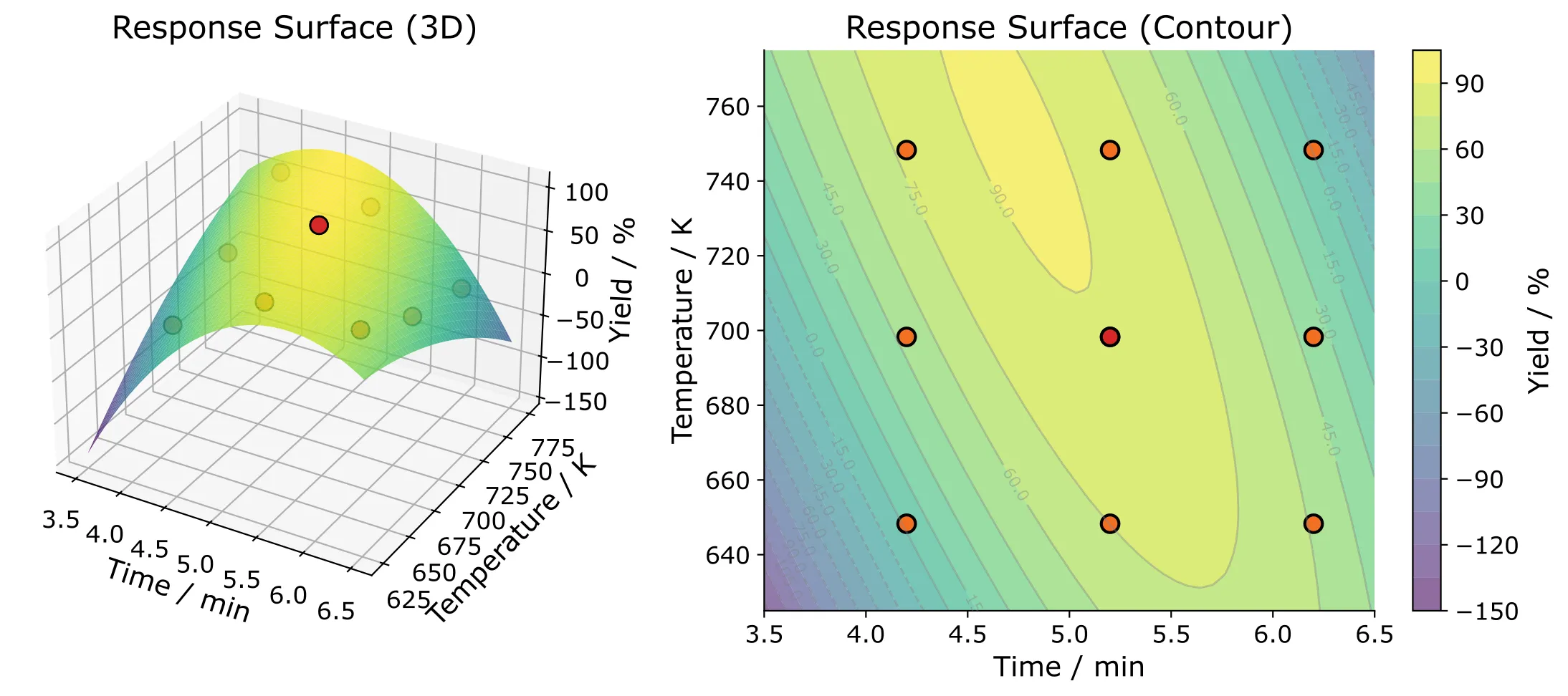
If you need a more accurate quantitative prediction close to the actual maximum, you could use a central composite design in the new design region of interest to model a more accurate response surface like shown in Figure 3 below.
The design toolkit
As mentioned earlier, RSM is an iterative approach, which means different stages require different experimental designs:
Fractional Factorial Designs are efficient when you have many factors and want to screen them without burning through resources.
Full Factorial Designs are best when you have only a few factors (typically < 4). Using a fractional factorial design here would lead to significant confounding, making interpretation difficult.
Central Composite Designs (CCD) build on factorial designs by adding axial points that extend beyond the original factor ranges. This allows you to fit quadratic models and get a more accurate representation of the local response surface.
Box-Behnken Designs are another option for second-order models. They’re efficient, especially if you have many factors. However, they’re less suited for the sequential nature of RSM because they don’t build naturally on factorial designs.
Limitations of RSM
Of course, RSM also has some important limitations. It’s a local optimization method and cannot model highly complex or global surfaces.
RSM also relies heavily on experimenter judgment. You decide when to move, where to move, and when to stop. There’s no autopilot. If you misjudge the situation, you might miss the real optimum.
Another challenge: RSM doesn’t easily integrate historical or external data. If you have legacy experiments or results from different studies, they typically won’t fit cleanly into the sequential framework. You’re building models based on what you run during the RSM process, not on everything you’ve ever done.
Bayesian Optimization is much better at doing that.
Some practicalities
- Using coded variables
I’ve been showing the natural units in my examples. However, I did all the calculations with coded factor levels. So instead of 750 and 850 K, I used “−1” and “+1.” Coding ensures all predictors are comparable and prevents one factor from dominating the regression simply because of scale differences.
- Handling Categorical variables
Categorical variables are tricky, but they occur often. Say you’re using different catalysts. You can label them as −1 and +1, but there’s no such thing as catalyst 0.5 or 0. That means you can’t smoothly move between levels the way RSM normally expects.
In practice, you usually have to find the optimal region for one catalyst, and then repeat the process for the next. Not very elegant because you also can’t necessarily assume that the best settings for catalyst A will also work for catalyst B.
That’s why categorical variables are difficult to handle, and whenever possible, it’s better to convert them into something numerical. Instead of using catalyst names, could you use a measurable property? Maybe Hansen Solubility Parameters for solvents, molecular weight for polymers, acidity, viscosity… something you can actually model?
Key Takeaway
That’s it. The key takeaway here is that RSM is a sequential approach, and it’s not perfect. It’s only an approximation, very rough in the beginning, and then you try to refine it as you go.
Think of it as a conversation with your process. You ask a question (run an experiment), listen to the answer (fit a model), make a move (follow the path), and ask again. Each cycle brings you closer to the optimum.
The key is patience and discipline. Don’t try to solve everything in one experiment. Don’t assume your first model is perfect. Trust the process, follow the data, and take it one step at a time.